Clastic rocks, including sand and gravel, are classified by geologists according to size, sorting, and distribution of particles, as well as chemical content of silica, feldspar, and calcite. It is often convenient for engineers to define clastic materials such as sand and gravel by particle size. Sand is defined with particle diameters ranging from 0.0625 mm to 2 mm. Gravel is defined with diameters ranging from 2 mm to an excess of 256 mm. Sand and gravel are defined as continuously graded unconsolidated materials (sediments) formed as a result of the natural disintegration of rocks.

Sand and gravel can be found in numerous depositional environments including alluvial (mudflows and streams), fluviatile (river), aeolian (wind), lacoustrine (lake), glacial, and beach/bar. Sand and gravel deposits can also occur without prior transportation in the form of residual (weathering) processes.

In the northern United States, many of the sand and gravel deposits were formed by glacial processes. Associated landforms include outwash plains, kames, eskers, and valley trains consisting of river terraces, flood plains, and channel deposits.

Alluvium is a broad term referring to all unconsolidated material formed in recent geological time under conditions other than subaqueous. Alluvial sand and gravel deposits are generally finer grained than glacial meltwater deposits, since present-day streams generally have less energy than meltwater streams and, therefore, less ability to transport large particles. In non-glaciated terrains, sand and gravel deposits are formed as sedimentary basins on talus slopes, and as alluvial deposits in flood plains and beds and terraces of rivers and streams.

The electrical properties and physical behavior of sand and gravel deposits will depend significantly on moisture content of the materials. Dry sand and gravel deposits will have a high electrical resistivity and a low seismic velocity. Saturated sand and gravel deposits will have a much lower resistivity and can be further influenced by the presence of salinity. Seismic velocity will probably be somewhat higher than that for water, which is about 1500 m/s.

The success of a geophysical survey will largely depend on the contrast in physical properties the sand and gravel deposit provides with its surroundings. The main methods used are resistivity methods. Seismic methods may be used to define the bedrock topography, but will probably not be used as an exploration technique for sand and gravel deposits. Likewise, Ground Penetrating Radar (GPR) methods may also be used if conditions permit, but should only be used for detailed surveys of existing deposits. Both of these methods are somewhat labor intensive and not appropriate for regional surveys.

Geophysical methods are used to better define existing sand and gravel deposits and to search for new sand and gravel deposits. If the goal is to better define an existing deposit, detailed geophysical surveys will probably be appropriate. These may include any of the methods mentioned earlier. If the goal is to find new deposits, the area for the search will dictate the investigation method. If very large areas are of interest, then airborne geophysical methods, such as resistivity mapping, may be appropriate. In this case, a search is made for resistivity highs. A brief description of airborne surveys is described later in this section of the website.

Understanding the relationship of the sand and gravel deposits with the bedrock may be important. Figure 156 shows where sand and gravel is deposited in a simple geology on top of horizontal bedrock. In this case, the effect of the bedrock on the geophysical data is constant over the section and does not unduly complicate the interpretation.

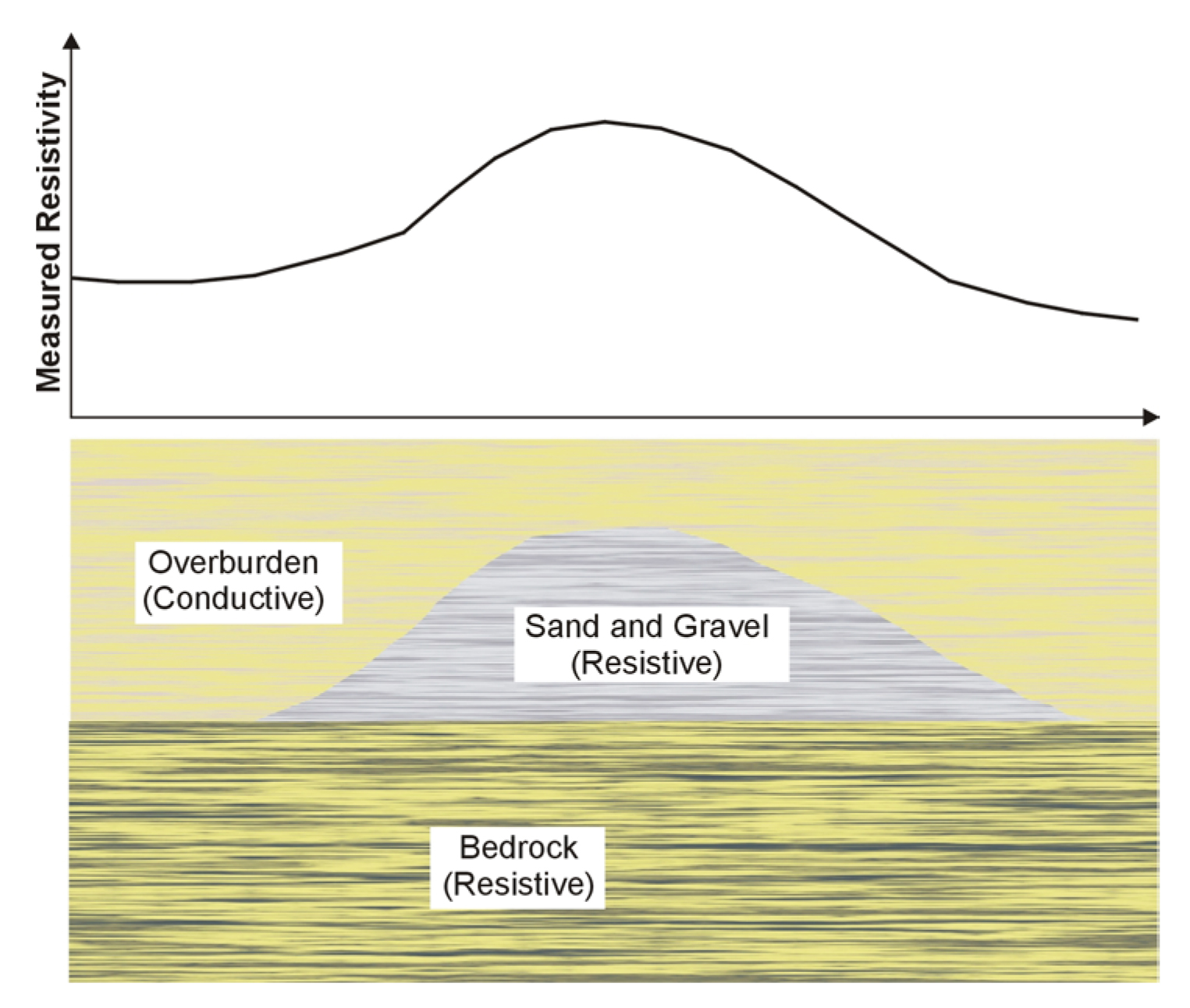
Figure 156. Sand and gravel - geological model.

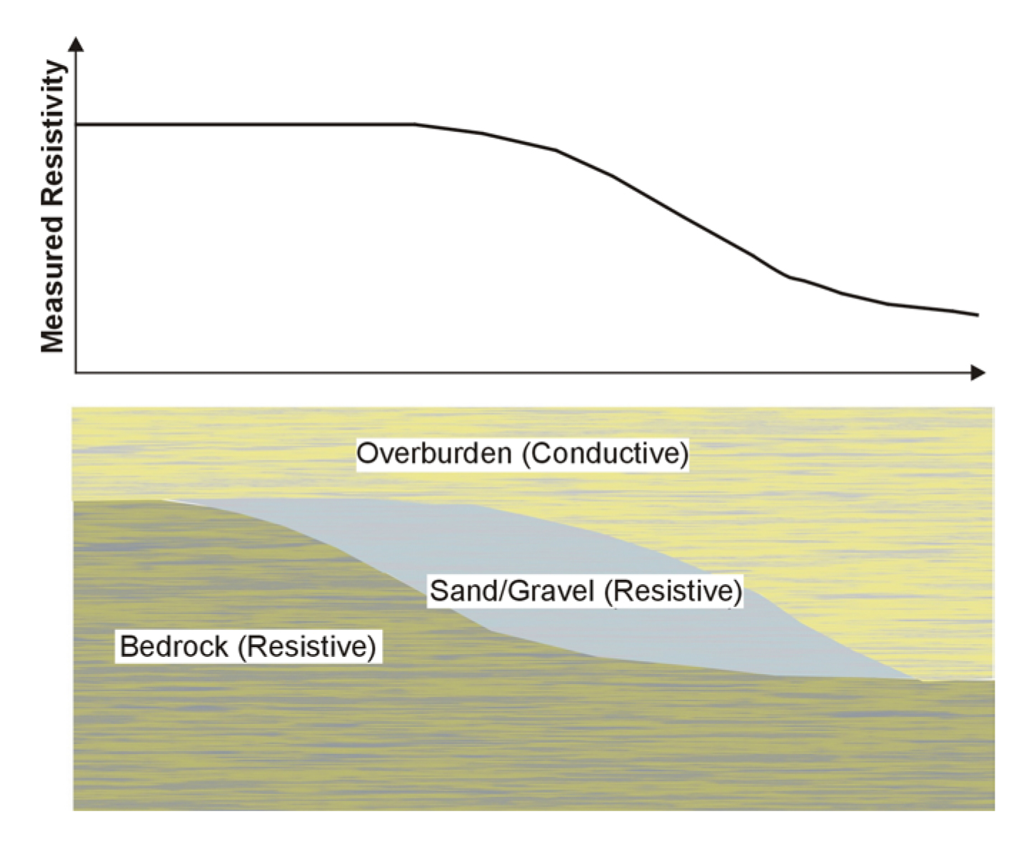
Figure 157. Sand and gravel deposit resting on bedrock slope.

However, figure 157 shows a more complex section where sand and gravel rests on a bedrock slope beneath an electrically conductive overburden. Both the sand and gravel and bedrock are assumed to be electrically resistive. Measurements of the electrical resistivity (or conductivity) over the sand and gravel deposit would not clearly define its position, since the bedrock and sand and gravel deposit are both electrically resistive. In fact, the resistivity measurements could be interpreted as simply indicating the bedrock topography. In this case, a different method is needed to define the bedrock surface. Since bedrock usually has a higher seismic velocity than either the sand and gravel or the overburden, seismic measurements could be used to map the bedrock surface. Knowing the bedrock topography, along with the resistivity profile, should allow an interpretation of the extent of the sand and gravel deposit to be made.

Methods

Resistivity; Soundings, and Traverses

Basic Concept: The resistivity of the ground is usually measured using one of several four-electrode arrays. These arrays are shown in figure 90. Resistivity is measured by passing electrical current into the ground using two electrodes and measuring the resulting voltage using two other electrodes.

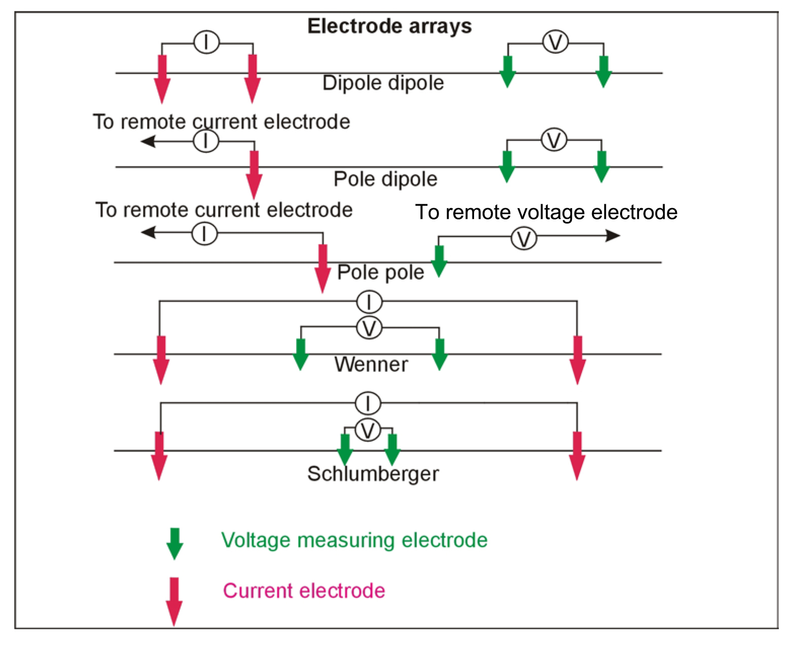
Figure 90. Electrode array used measuring resistivity.

These arrays are used for different types of resistivity surveys. The Schlumberger array is often used for resistivity soundings, as is the Wenner array. The pole-pole array provides the best signal, but is cumbersome because of the long wires required for the remote electrodes, and it is rarely used. The dipole-dipole array was originally used mostly by the mining industry for induced polarization surveys. Readings were taken using several different separations of the voltage and current dipoles providing measurements of the variation of resistivity with depth. Long lines of data were recorded requiring many readings. This array has now become common for resistivity surveys using automated resistivity systems. If more signal (voltage) is needed than can be provided with the dipole-dipole array, the pole-dipole array can be used.

Resistivity measurements using the Schlumberger array are illustrated in figure 91. By enlarging the electrode spacing, deeper layers are imaged. If resistivity measurements from a number of electrode spacings are used, a plot of measured resistivity against electrode spacing can be drawn. This is called a resistivity sounding curve. At large electrode spacings, the measured resistivity is close to that of the bedrock, i.e. Rho2 (figure 91b). When the electrode spacings are small, the measured resistivity is close to that of the overburden, i.e. Rho1 (figure 91b).

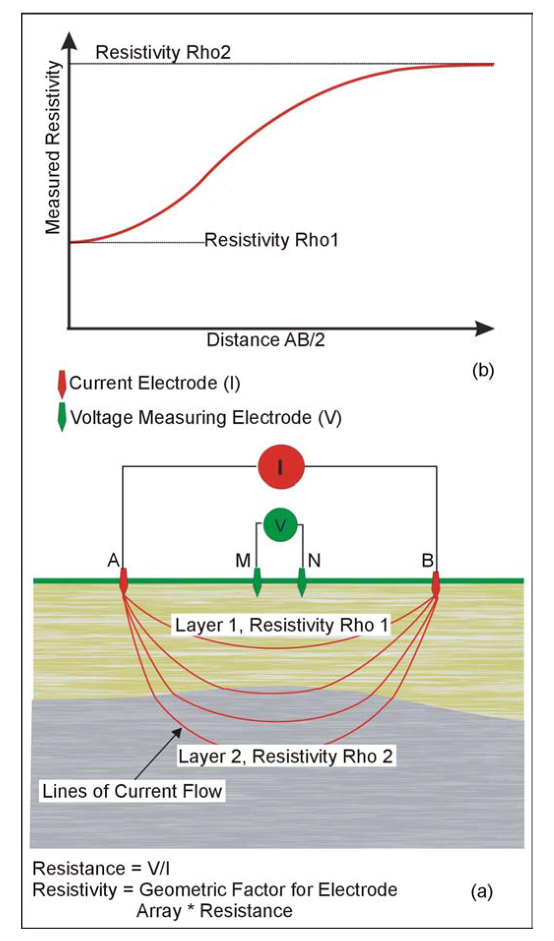
Figure 91. Electrode array for measuring the resistivity of the ground (a), and a resistivity sound curve (b).

Data Acquisition: Resistivity measurements can be made along traverses using one electrode spacing, thus providing the lateral variation of resistivity. However, this method is rarely used and will not be discussed further, since electromagnetic techniques are available to measure conductivity (inverse of resistivity) that do not require ground contact and are much more efficient. However, the resistivity method is still used to obtain the vertical distribution of resistivity, called resistivity soundings, as discussed previously.

Data Processing: The most important thing is to remove bad data points.

Data Interpretation: Resistivity sounding curves can be interpreted to give the resistivities and thickness of the layers imaged under the sounding site. This is done using software that modifies an initial model input by the interpreter such that the model data match the field data. The data are usually checked for bad data points before interpreting.

Resistivity soundings could be used to measure the vertical distribution of resistivity over an area of interest. If the method were used to search for unsaturated sand and gravel, the objective would probably be to search for electrically resistive regions. In addition, if the bedrock provided a good resistivity contrast with the overburden and was imaged by the resistivity soundings, then the bedrock depth could also be obtained. If the area was saturated, then the resistivity contrast with the host rocks will likely be smaller.

Advantages: Resistivity soundings prove an efficient and effective method of measuring the resistivity of the ground down to depths of 100 feet or more.

Limitations: The method is quite labor intensive since four electrodes have to be inserted into the ground for every resistivity reading. A sounding curve may have 15 measured resistivities, depending on the complexity of the geologic section.

The measured resistivity is influenced by nearby metal fences and other grounded metal objects. If the ground is hard then more effort is needed to place the electrodes and water may need to be poured on to the electrodes to improve the electrical contact between the electrode and ground.

Automated Resistivity Systems

Basic Concept: Resistivity measurements can be taken using recently developed instruments that use addressable electrodes, called Automated Resistivity systems. With these systems, the required electrodes are planted prior to recording data, and the wires between all of the electrodes and the recorder are also connected. The recorder is programmed with the electrode array to be used along with other data recording parameters and instructed to take the measurements. The system automatically records the data according to these preset instructions, automatically switching between electrodes as needed. One such system is called a Sting/Swift system illustrated in figure 201.

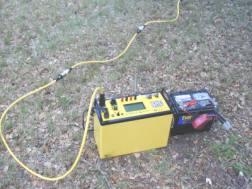
Figure 201. SuperSting R1 IP resistivity meter. (Advanced Geosciences, Inc.)

This system provides detailed resistivity data and is probably not suited to explore large areas. If large areas are to be explored, other methods should probably be used as reconnaissance techniques, and this technique used for detailed analysis of interesting areas. Conductivity methods, discussed in the next section, may be appropriate for reconnaissance.

Data Acquisition: As discussed previously, data are recorded automatically by the instrument. If long lines are required to be recorded, the system is moved along the line a specified distance and the data recording procedure repeated. The data are plotted as sections showing the variation of resistivity with depth, as illustrated in figure 202.

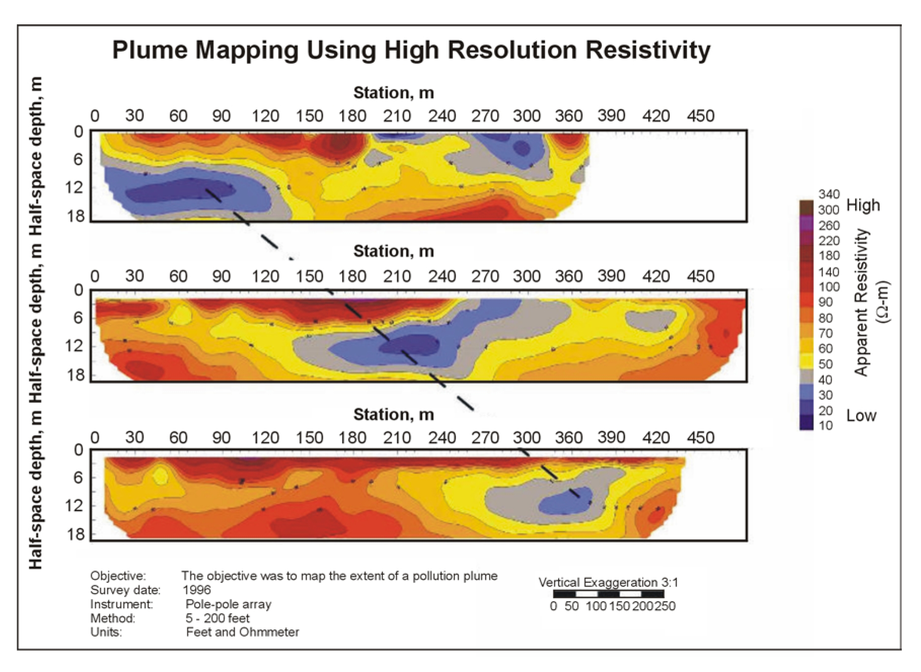
Figure 202. Example data recorded with the Sting-Swift System. (Advanced Geoscience, Inc.)

Data Processing: Little processing is applied to the measured resistivity data, although bad data points may need to be removed.

Data Interpretation: Interpretation is done using inversion software. The software iteratively modifies a preliminary model input by the interpreter until the calculated model data fit the field data, a process called inversion.

Advantages: Automated resistivity systems proved an efficient system for recording field data.

Limitations: The methods that require electrodes are difficult to use in areas where the surface of the ground is hard, such as concrete or asphalt-covered areas or frozen ground. In addition, if the contact between the electrode and ground is poor, as in rocky soil, water may need to be poured on the electrodes to lower the resistance to ground of the electrodes.

If data are only recorded along a single line, lateral variations in resistivity normal to the line will not be accounted for. However, recording lines parallel to each other can rectify this problem. In addition, three-dimensional surveys can be recorded. Cultural features such as power lines, fences, and other metal features may provide false anomalies. These cultural features will have to be noted in the field and accounted for in the interpretation.

Another instrument for measuring the resistivity is called the Ohm-Mapper, manufactured by Geometrics. This instrument has a series of electrodes on a cable that is dragged at a slow pace along the ground. Current is induced into the ground, and the resulting voltages measured. The electrodes are capacitively coupled to the ground and both transmit current into the ground and measure the resulting voltage. The Ohm-Mapper instrument being towed along the ground surface is shown in figure 200.

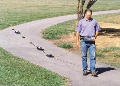
Figure 200. The Ohm-Mapper. (Geometrics, Inc.)

The instrument appears to provide the best results in resistive environments and is generally limited to fairly shallow surveys of less than about 10 m.

Conductivity Measurements

Basic Concept: Electrical conductivity measurements can be made over a larger area as a reconnaissance tool and a map produced showing the conductivity down to a particular depth. These data can be used to locate anomalous conductivity zones that may correspond to sand and gravel deposits.

Conductivity measurements can also be taken to map the vertical distribution of layers under the sounding site. The method used for this purpose is called Time Domain Electromagnetic Soundings (TDEM). However, this method is best suited to depths greater than 10 m in moderate-to-high conductivity sections and is less appropriate in resistive conditions. Thus, the method is unlikely to be frequently used for sand and gravel exploration unless thick deposits are expected. This method is probably more appropriate for mapping existing deposits than exploring large areas for new deposits.

Ground conductivity measurements are recorded using several instruments that use electromagnetic methods. The choice of which instrument to use generally depends on the depth of investigation desired. Instruments commonly used include the EM38, EM31, EM34, and GEM2. Since the EM38 has a maximum exploration depth of about 1.5 m, it is not appropriate for sand and gravel exploration and is not discussed in this section of the website.

The EM31 has a depth of investigation to about 6 m, and the EM34 has a maximum depth of investigation to about 60 m. The depth of investigation of the GEM2 is advertised to be 30 to 50 m in resistive terrain (>1,000 ohm-m) and 20 to 30 m in conductive terrain (<100 ohm-m).

Electromagnetic instruments that measure ground conductivity use two coplanar coils, one for the transmitter and the other for the receiver. The transmitter coil produces an electromagnetic field, oscillating at less than 10 kHz (EM31 and EM34) and from 330 Hz to 24 kHz for the GEM2. This oscillating electromagnetic field produces secondary currents in conductive materials in the ground. The amplitude of these secondary currents depends on the conductivity of the material. The secondary currents produce a secondary electromagnetic field that is recorded by the receiver coil.

These instruments can be used with the planes of the coils held parallel to the ground (vertical dipole mode) or perpendicular to the ground (horizontal dipole mode). The investigation depth is greatest in the vertical dipole mode and least in the horizontal dipole mode. In addition, in the vertical dipole mode, the conductivity readings are insensitive to near-surface conductivity changes, whereas in the horizontal dipole mode, the readings are significantly influenced by near-surface conductivity changes. Figure 183 shows the EM31 instrument being used in vertical dipole mode. Figure 197 shows the EM34 being used in horizontal dipole mode, and the GEM3 instrument is shown in figure 219.

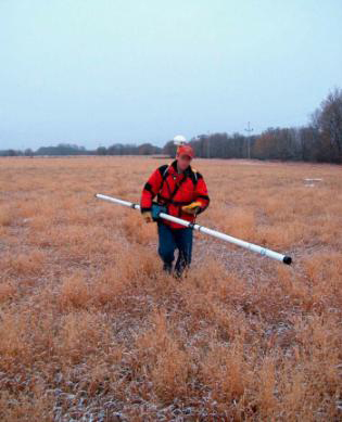
Figure 183. The EM31-Mk2 instrument. (Geonics, Ltd.)

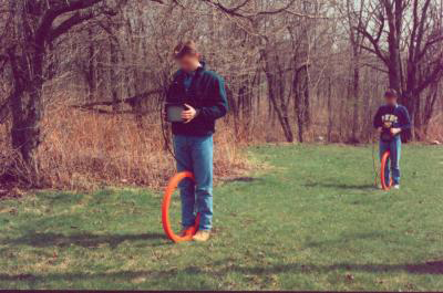
Figure 197. The EM34 being used in horizontal dipole mode. (Geonics, Ltd.)

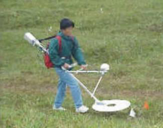
Figure 219. The GEM-3 electromagnetic instrument. (Geophex, Inc.)

The EM31 is effective to depths of about 6 m. If conductivity measurements are required to greater depths then the EM34 should be used. This instrument can be used to depths up to about 60 m. Three different separations of the two coils can be used providing six different depths of investigation (three coil separations and two modes for each separation). However, as the depth of investigation increases, the lateral resolution decreases. The EM34, unlike the EM31, requires two people to operate. Data recording is also much slower than with the EM31. All of these instruments measure the bulk electrical conductivity of the ground. Since the conductivity of several different layers may be included in the conductivity measure, the correct technical term for the measured conductivity is apparent conductivity. The term terrain conductivity is also often used to describe the conductivity values. When discussing data from these instruments in this website, conductivity or measured conductivity is understood to mean apparent (or terrain) conductivity.

Data Acquisition: Surveys are conducted by taking readings along lines crossing the area of interest. These lines need to be surveyed in order to have spatial coordinates recorded. Readings are taken either at defined stations or on a timed basis, e.g., every second (EM31). The mode in which the instruments are used depends on the target depth and the objectives. The instruments store the data in memory, allowing the data to be downloaded to a computer later. Surveys can be conducted using different coil spacings (EM34) and modes (EM31 and EM34, horizontal and vertical dipole modes) providing different investigation depths.

Data Processing: Data processing involves assigning coordinates to each data point. These data are then gridded, contoured, and plotted, producing a map of the measured conductivity of the site.

Data Interpretation: Interpretation is done from this map. Generally, this will involve searching for areas of low electrical conductivity (high resistivity). These areas will be the most likely places to find sand and gravel deposits.

In cases where data have been recorded with different modes and coil spacings, a layered model can be produced using inversion software.

Advantages: The EM31 and EM34 both provide efficient methods for mapping lateral changes in conductivity.

Limitations: The instruments transmit an electromagnetic field to produce secondary currents in conductive regions of the ground. However, currents are also generated in metal objects on/in the ground, such as fences and pipelines. The electromagnetic fields from these objects are detected by the receiver coil, in addition to fields from geological targets, making interpretation of the data difficult.

Measurements of conductivity simply map the conductivity of the ground to the depth of investigation of the instrument. Complex geological situations, such as that illustrated in figure 157, cannot be interpreted from these data alone. Conductivity or resistivity measurements along a traverse using a single coil (conductivity) or electrode (resistivity) spacing do not provide meaningful depth information beyond the broad investigation depth information provided by the coil or electrode spacing. Thus, the measurements could be responding to the bedrock geology as well as the overburden. Other methods, such as electrical soundings or seismic refraction will typically be needed to map the bedrock depths, allowing for a more comprehensive interpretation.

Figure 157. Sand and gravel deposit resting on bedrock slope.

Time Domain Electromagnetic Soundings

Basic Concept: Time Domain Electromagnetic (TDEM) soundings are another method for obtaining the vertical distribution of the resistivity of the ground. This method is particularly well suited to mapping conductive layers. To a significant degree, this method has now superseded the resistivity sounding method since it requires less work for a given investigation depth and generally provides more precise depth estimates. However, resistivity soundings are still useful for shallow investigations or when resistive targets are sought. Figure 120 provides a conceptual drawing of the TDEM method.

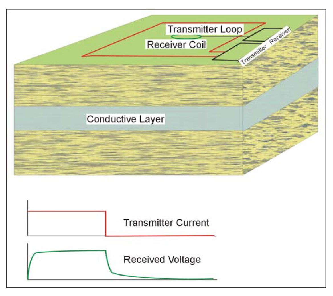
Figure 120. Time Domain Electromagnetic Sounding.

TDEM soundings are an electromagnetic method used to provide the vertical distribution of resistivity within the ground. A square loop of wire is laid on the ground surface with a side length that is about half of the desired depth of investigation. A receiver coil is placed in the center of the transmitter loop. Electrical current is passed through the transmitter loop and then quickly turned off. This sudden change in the transmitter current causes secondary currents to be generated in the ground. These currents decay for longer times in more conductive rocks. The relationship between the time after the transmitter current has turned off (delay time), layer depth, and conductivity is quite complex, although generally, longer delay times are needed to investigate to greater depths.

The voltage measured by the receiver coil does not decay instantly to zero when the current is turned off, but continues to decay for some time. This decaying voltage is caused by the decaying secondary electrical currents in the ground. The receiver measures this voltage, which is then converted to measured resistivity. A plot is made of the measured resistivity against the delay time, as illustrated in figure 121.

The resistivity sounding curve shown in figure 121 illustrates the curve that would be obtained over three-layered ground. The near-surface layer is fairly resistive. This is followed by a layer having a much lower resistivity (higher conductivity) and causes the measured resistivity values to decrease. The third layer is again resistive.

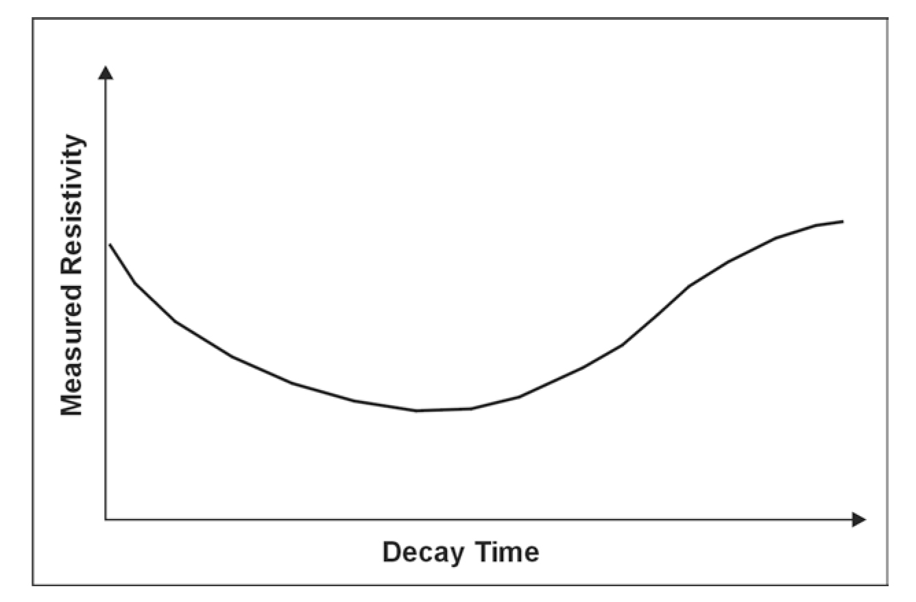
Figure 121. A Time Domain Electromagnetic Sounding curve.

Data Acquisition: The field layout for a TDEM survey is described previously. Switched current is passed through the transmitter loop, and the resulting voltage is measured by the receiver coil. The switching and measuring procedure is repeated many times, allowing the resulting voltages to be stacked and improving the signal-to-noise ratio. Soundings are conducted at additional locations until the area of interest has been covered. Sounding curves are plotted for each location showing the measured resistivity against decay time.

Data Processing: Little processing is applied to the data, although bad data points may sometimes be removed.

Data Interpretation: Sounding curves are interpreted using computer software to provide a model showing the layer resistivities and thickness. The interpreter inputs a preliminary model into this software program, which then calculates the sounding curve for this model. It adjusts the model and calculates a new sounding curve that better fits the field data. This process, called inversion, is repeated until a satisfactory fit is obtained between the model and the field data. The sounding curve shown in figure 121 illustrates the type of curve expected over a conductive shale layer.

Advantages: TDEM soundings are an efficient method for investigating the vertical distribution of ground resistivity. Generally, the method is better suited to mapping conductive formations rather than resistive formations. However, bedrock is usually more resistive than the overburden, and, provided the bedrock is not too shallow or resistive, the TDEM method should be applicable.

Limitations: The interpretation of the TDEM method assumes that the layers are horizontal and homogeneous; incorrect interpreted resistivities and/or depths will result if this is not the case. However, this should not be a serious problem for mapping bedrock depths.

Probably the most troublesome aspect of data recording is the influence of fences, power lines, and other cultural features at the survey site.

Airborne Resistivity

Basic Concept: Airborne resistivity methods may be appropriate when large areas are to be explored for sand and gravel deposits. Airborne surveys can be conducted using either a fixed wing aircraft or a helicopter.

Figures 158 and 159 show fixed wing aircraft and helicopter conductivity (resistivity) measuring systems. In the fixed wing aircraft, the transmitter loop is the wire that can be seen encircling the aircraft and attached to the nose, wings, and tail. The electromagnetic instrumentation for the helicopter system is mounted in a cylindrical boom and attached to the helicopter using a long cable.

Specialized equipment mounted in small planes or helicopters is used to collect data on the magnetism or electromagnetic conductivity of rock over large areas.

Data Acquisition: Airborne geophysical surveys require very specialized knowledge and only a very brief discussion is presented in this web manual.

Most airborne surveys now use GPS for navigation. Lines are planned before surveying begins and transmitted to the pilot during flights using electronic instrumentation that guides him to the correct line to be surveyed.

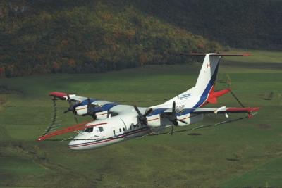
Figure 158. Fixed wing airborne conductivity system. (Fugro Airborne Surveys)

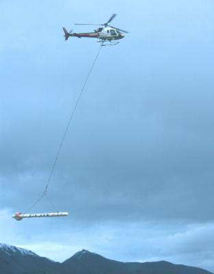
Figure 159. Helicopter conductivity measuring system. (Fugro Airborne Surveys and John Holland, ERA Helicopters)

Data Processing: Depending on the type of survey conducted, a significant amount of processing may be required to correct for various factors. The final product is usually a map showing the conductivity (or resistivity) of the area surveyed.

Data Interpretation: The data is interpreted by observing the changes in resistivity and searching for more resistive areas. The results from an airborne survey for sand and gravel are illustrated in figures 160 and 161.

Figure 160 shows the high resistivity areas that were found to be sand and gravel deposits. A section across anomaly A has been drawn, showing the measured resistivity and the drill results and is presented in figure 161.

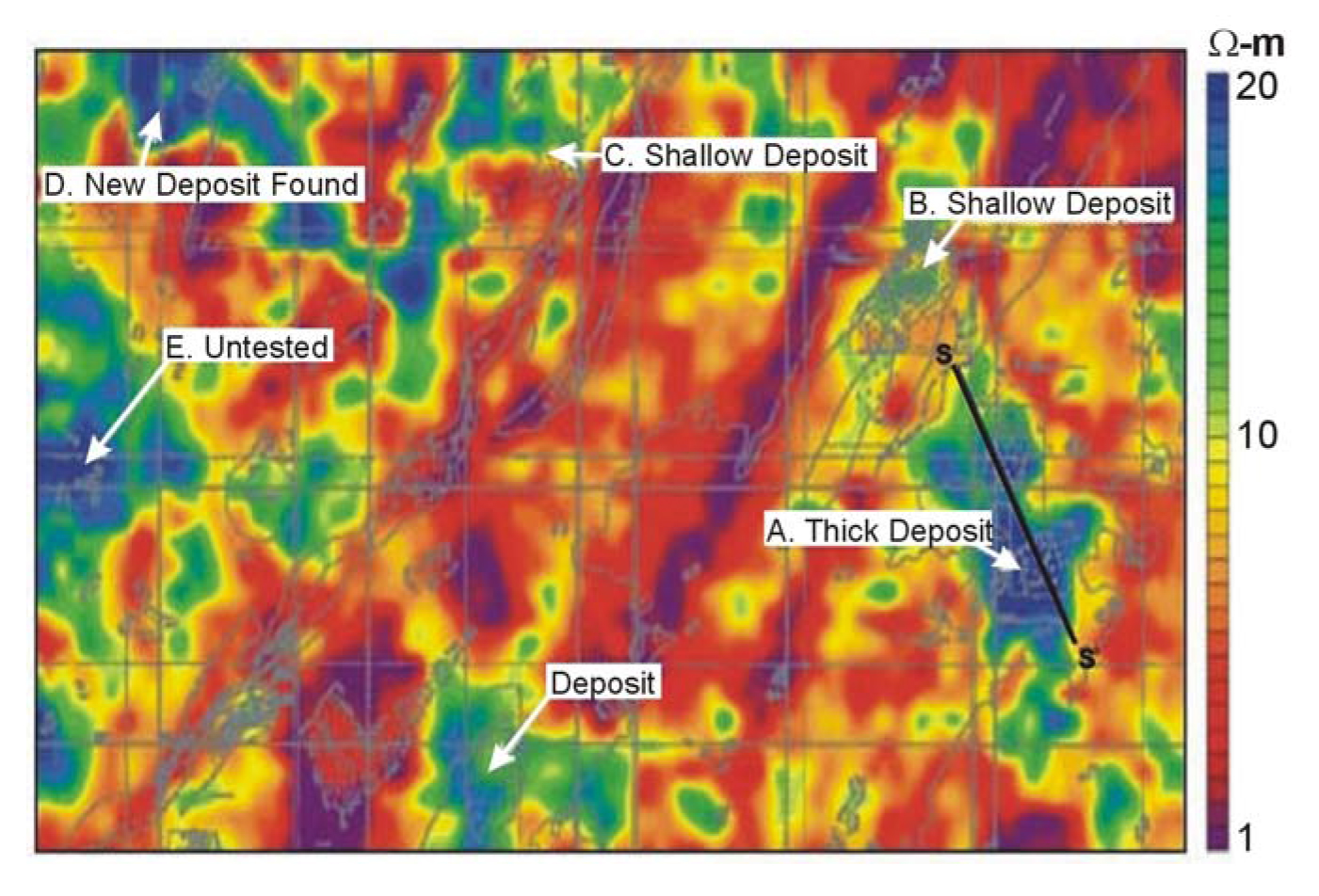
Figure 160. Results from an airborne survey for sand and gravel. (Fugro Airborne Surveys)

This survey was flown and processed by Fugro Airborne Surveys over an area in Saskatchewan, Canada.

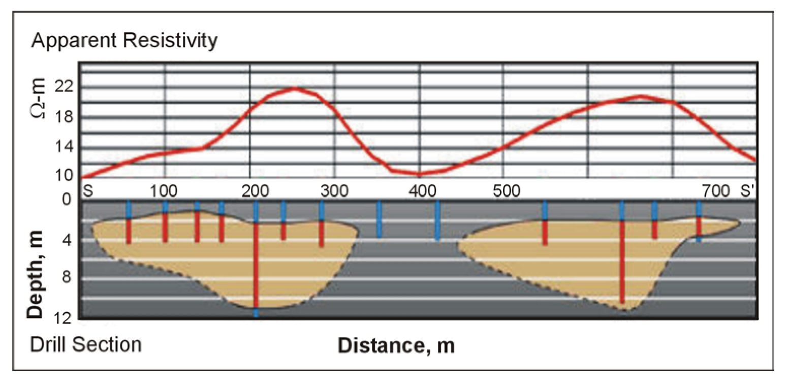
Figure 161. Section showing drill results and resistivity values over a sand and gravel deposit. (Fugro Airborne Surveys)

Seismic Refraction

Basic Concept: Seismic refraction methods will most likely be used to better define the boundaries of existing deposits. They may be used to map the bedrock depths over an area of interest for sand and gravel deposits. Areas where the bedrock is deepest will be of greatest interest. This method may be useful for geologic sections illustrated in figure 157.

Figure 157. Sand and gravel - geological model.

Seismic refraction is one of the most commonly used methods for finding bedrock depths, especially for depths of less than 30 m. The method requires a seismic energy source, usually a hammer for depths of less than 15 m and black powder ges for depths to 30 m. The seismic waves then penetrate the overburden and refract along the bedrock surface. While they are traveling along this surface, they continually refract seismic waves back to the ground surface. These are detected by geophones placed on the ground surface. Both compressional waves and shear waves can be used in the seismic refraction method, although compressional waves are most commonly used. Figure 114a shows the layout of the instrument, the main seismic waves involved, and the resulting time distance graph.

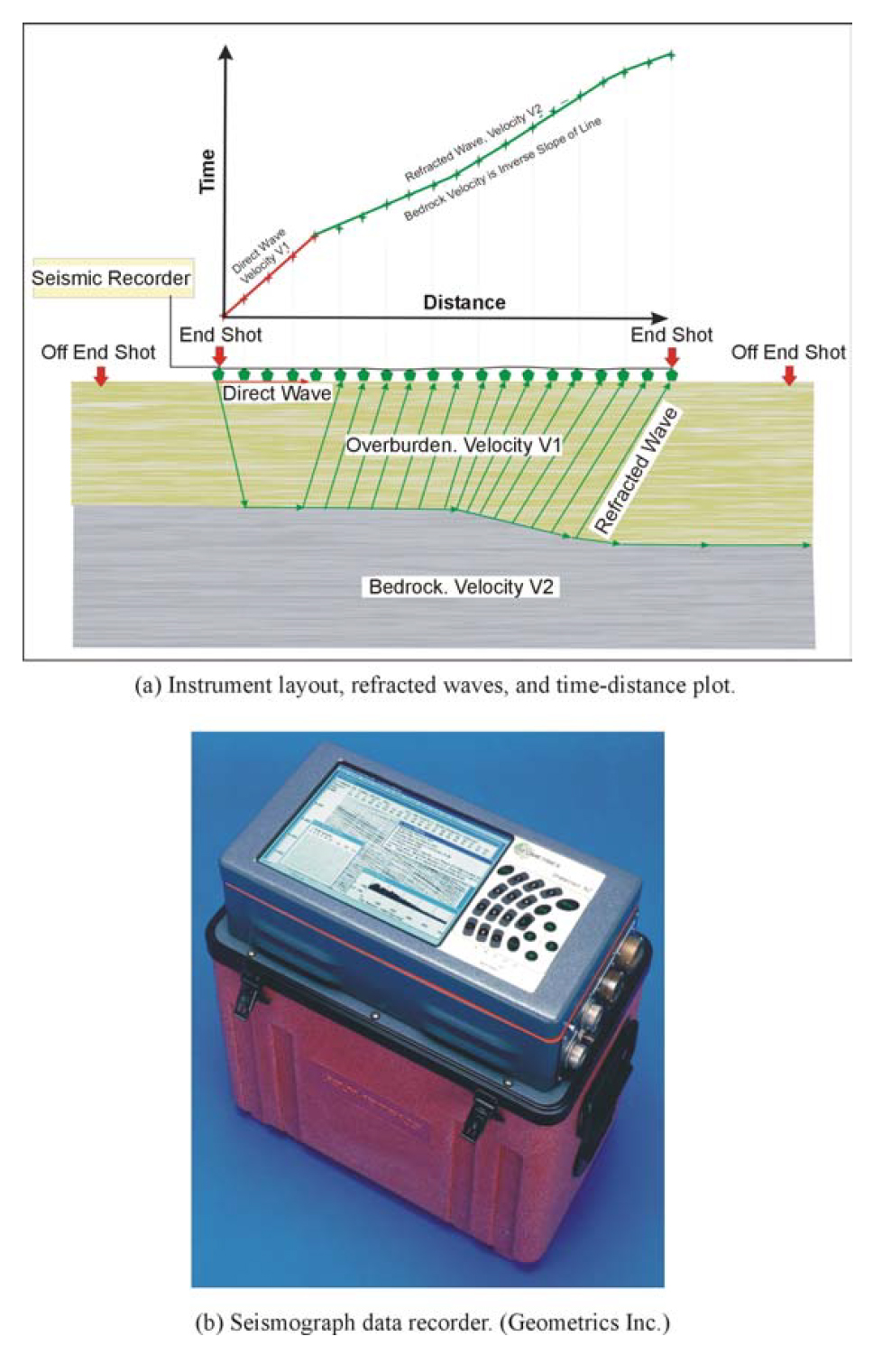
Figure 114. Seismic Refraction: field set up and data recorder.

Data Acquisition: The design of a seismic refraction survey requires a good understanding of the expected bedrock and overburden. With this knowledge, velocities can be assigned to these features and a model developed that will show the parameters of the seismic spread best suited for a successful survey. These parameters include the length of the geophone spread, the spacing between the geophones, the expected first break arrival times at each of the geophones, and the best locations for the off-end shots. Knowing the expected first break arrival times is also helpful in the field, where field arrival times that correspond fairly well to expected times help to confirm that the spread layout has been appropriately planned, and that the target layer is being imaged.

Data Processing: The first step in processing/interpreting refraction seismic data is to pick the arrival times of the seismic signal, called first break picking. A plot is then made showing the arrival times against distance between the shot and geophone, called a time-distance graph. An example of such a graph for a two-layered ground (overburden and refractor) is shown in figure 114a.

The time distance plot shows the waves arriving at the geophones directly from the shot (V1) and the refracted waves that arrive ahead of the direct waves (V2). These refracted waves have traveled a sufficient distance along the higher speed refractor (bedrock) to overtake the direct wave arrivals.

Data Interpretation: One of the most common methods of refraction interpretation is Generalized Reciprocal Method (GRM) that is described in detail in the Geophysical Methods section. A brief, and simplified, description of the GRM method is presented below. Figure 115 shows the basic rays used for this interpretation.

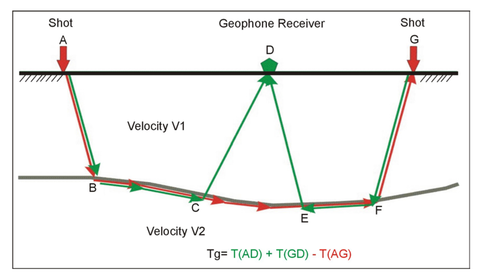
Figure 115. Basic Generalized Reciprocal method interpretation.

The objective is to find the depth to the bedrock under the geophone at D. This is done using the following simple calculations. The travel times from the shots at A and G to the geophone at D are added together (T1). The travel time from the shot at A to the geophone at G is then subtracted from T1. Figure 116 shows the remaining waves after the above calculations have been performed. These are the travel times from C to D added to the travel times from E to D, subtracting the travel time from C to E. The sum of these travel times can be shown to be approximately the travel time from the bedrock at H to the geophone at D. Since the velocity of the overburden layer can be found from the time distance graph, the distance from H to D can be found giving the bedrock depth.

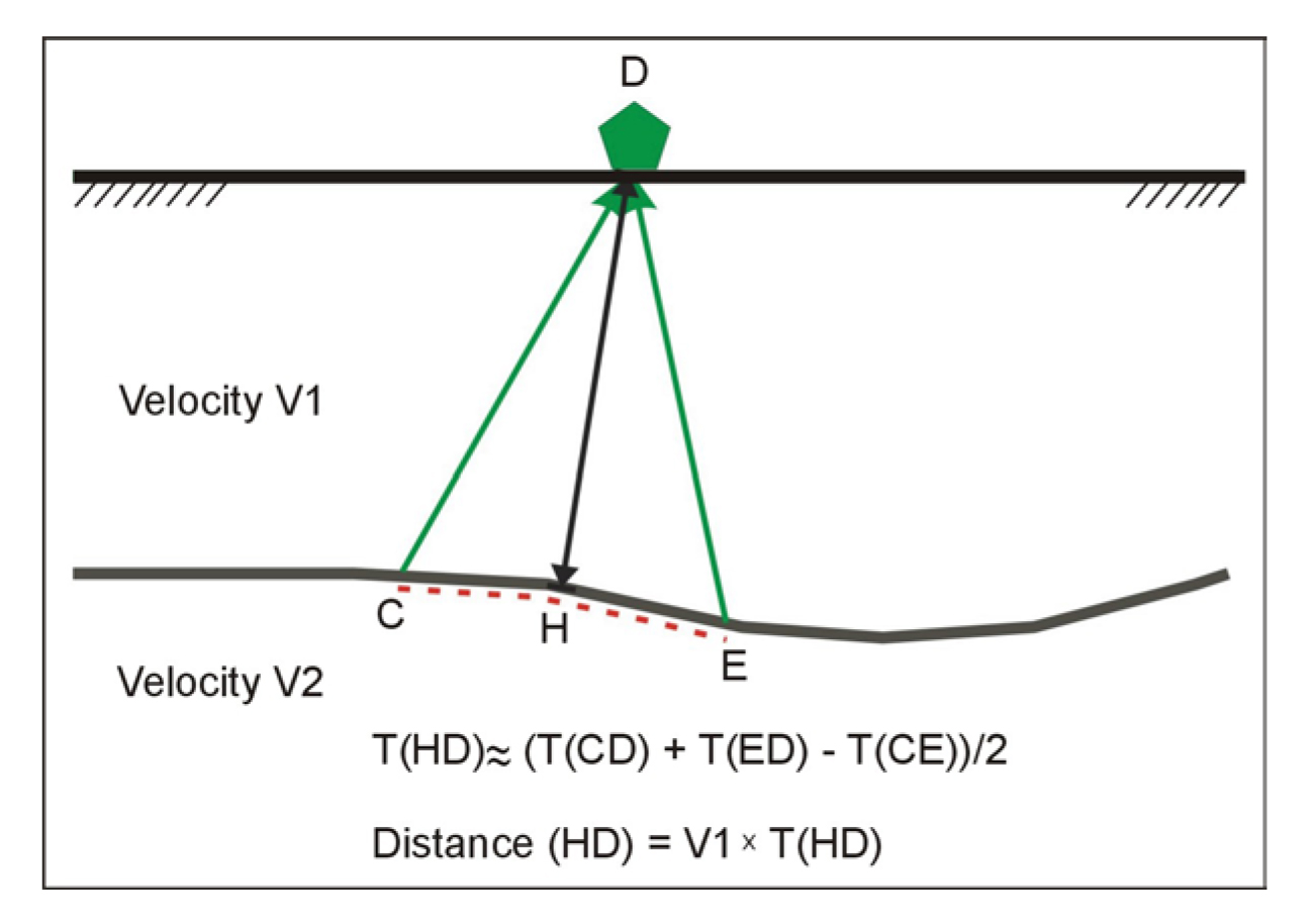
Figure 116. Generalized Reciprocal method interpretation.

Advantages: The seismic refraction method may be useful to map the thickness of a sand and gravel deposit if the base has a higher velocity than the sand and gravel and provides reasonably accurate depth estimates.

Limitations: Probably the most restrictive limitation is that each of the successively deeper refractors must have a higher velocity than the shallower refractor. However, for determining bedrock depths, this is probably not a significant limitation since the bedrock usually has a higher velocity than the overburden.

If the water table is in the overburden and close to the bedrock, this may obscure the bedrock arrivals since bedrock has a higher velocity than unsaturated soils. This could also limit the velocity difference between the bedrock and saturated overburden, making it difficult to observe the bedrock with the seismic refraction method.

Local noise, for example traffic, may obscure the refractions from the bedrock. This can be overcome by using larger impact sources or by repeating the impact at a common shot point several times and stacking the received signals. In addition, since some of the noise travels as airwaves, covering the geophones with sound absorbing material may also help to dampen the received noise.

Ground Penetrating Radar

Basic Concept: The Ground Penetrating Radar (GPR) method is not expected to be commonly used for exploration of sand and gravel deposits. However, there may be occasions where its use is justified, and it is described here for that reason. If the method is used, it seems likely that the target will be the bedrock depth.

GPR can be used where the bedrock is expected to be shallow, and the overburden is unsaturated and contains no clay or silt. If these conditions exist, penetration depths may be a few meters. The GPR instrument consists of a recorder and a transmitting and receiving antenna. Different antennas provide different frequencies, which vary between 25 MHz to 2700 MHz. Lower frequencies provide greater depth penetration but lower resolution. Figure 111 provides a drawing illustrating the GPR system. The transmitter provides the high frequency electromagnetic signals, which penetrate the ground and are reflected from objects and boundaries providing a different dielectric constant from that of the overburden. The reflected waves are detected by the receiver and stored in memory.

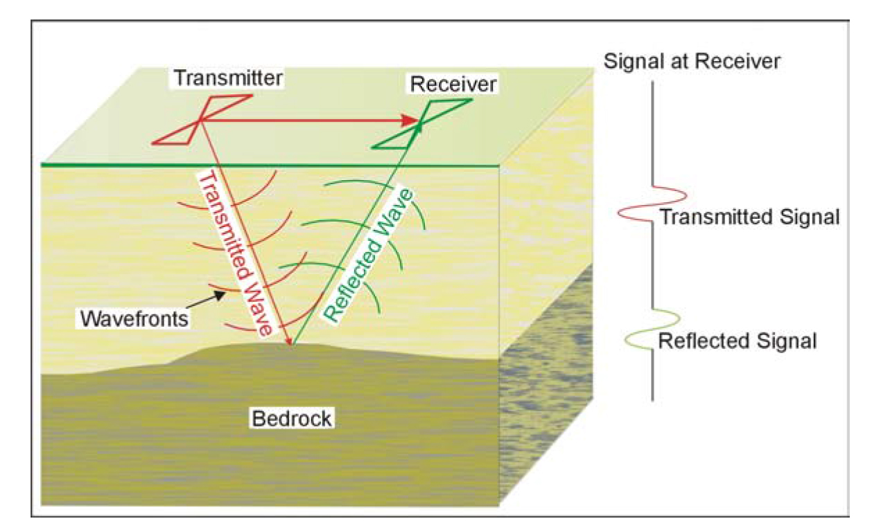
Figure 111. Ground Penetrating Radar system.

Figure 112 shows typical GPR equipment. This picture shows the display and the controls for the equipment.

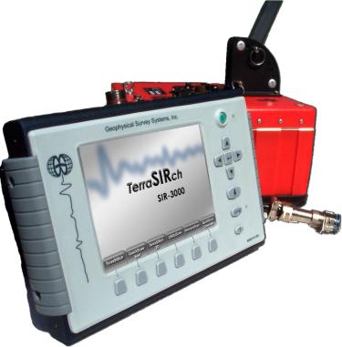
Figure 112. Ground Penetrating Radar instrument. (Geophysical Survey Systems, Inc.)

Figure 113 shows a 100 MHz antenna being pulled across the ground as the survey is conducted. This is a fairly low-frequency antenna and can provide penetration to about 20 m, depending on the ground conditions.

Data Acquisition: GPR surveys are conducted by pulling the antenna across the ground surface at a normal walking pace, as shown in figure 113. The recorder stores the data as well as presenting a picture of the recorded data on a screen. Surveys for sand and gravel are likely to be done using the lower frequency antenna since depth of penetration is more important than resolution.

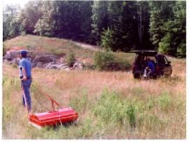
Figure 113. Ground Penetrating Radar antenna (100 MHz)

Data Processing: It is possible to process the data, much like the processing done on single-channel reflection seismic data. Processes that may be applied include distance normalization, horizontal scaling (stacking), vertical and horizontal filtering, velocity corrections, and migration. However, depending on the data quality, this may not be done since the field records may be all that is needed to observe the bedrock.

Data Interpretation: The data are usually interpreted visually. If the target is the bedrock, a horizontal, or sub horizontal, reflector would be observed at the expected depth. To calculate the depth to the bedrock, the speed of the GPR signal in the soil at the site needs to be obtained. This can be estimated from textbook speeds for typical soil types, or it can be obtained in the field by conducting a small traverse across a buried feature whose depth is known.

Advantages: The method is easy to use and provides a visual display of the results as the survey progresses. Different antenna, providing different penetration depths and resolution, can easily be tested.

Limitations: Probably the most limiting factor for GPR surveys is that their success is very site specific and depends on having a contrast in the dielectric properties of the target compared to the host overburden along with sufficient depth penetration to reach the target. The method is slow compared to recording conductivity data with the EM31 or EM34. It is more suited to defining the extent of existing sand and gravel deposits and will probably find little use in exploring new areas.

If the sand and gravel deposit contains a significant amount of cobbles, these may reflect and scatter the GPR signal, resulting in only a small amount of energy reaching the bedrock surface. In this case, the bedrock surface may not be observed with this method.