Lithology is a description of rocks, especially sedimentary rocks, mostly from hand specimens and outcrops. This description includes the color, structure, mineralogical composition, and grain size. Geophysical methods measure the physical properties of rocks, including seismic wave velocity, resistivity, induced polarization, magnetization, and, at shallow depths, dielectric properties. To use geophysical methods to map lithology, there has to be some relation between the lithological parameters and the physical properties of the rock.
The two lithological parameters that can be most readily correlated from geophysical measurements are structure and grain size. Color cannot be translated from geophysical methods to a physical property. Mineralogical composition is loosely related to seismic velocity, although this relationship is probably quite complex. The only minerals that can be detected directly using geophysical methods are magnetite and metallic sulfides, such as pyrite.
The distribution of grain size within a rock is related to porosity. Porosity is the ratio between the volume of pore space and the total volume of rock. A uniform wide grain size distribution usually results in a lower porosity than a narrow distribution, since the smaller grains can fill in the spaces between the larger grains. The critical grain size cannot generally be readily determined from porosity. Porosity can provide an indicator of the relative grain size distribution (wide or narrow) since materials with wide grain size distributions will typically have less pore space or lower porosity than materials with narrow distributions. Structure is probably related to seismic velocity and less to resistivity. Seismic velocity is strongly related to density, with denser rocks having a higher seismic velocity. However, since there is a considerable overlap of densities for different rock types, it is difficult to predict rock type, and hence lithology, from density. Likewise, the resistivity of any particular rock type varies over a wide range, and there is a large overlap of rock types having similar resistivities. Probably the most definitive relationship is between seismic velocity and porosity, although, as with density, there is a large overlap of different rock types with similar velocities. Figures 145 and 146 show the resistivity and seismic velocity of numerous rock types and illustrates the overlap in rock type for both resistivity and velocity.
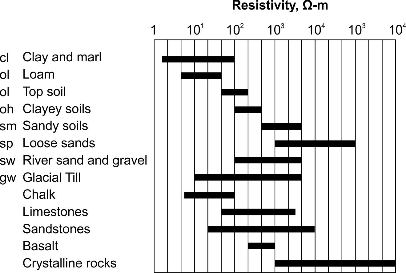
Figure 145. Resistivities of different rock types. (From TN5, Electrical Conductivity of Soils and Rocks, Geonics Ltd)
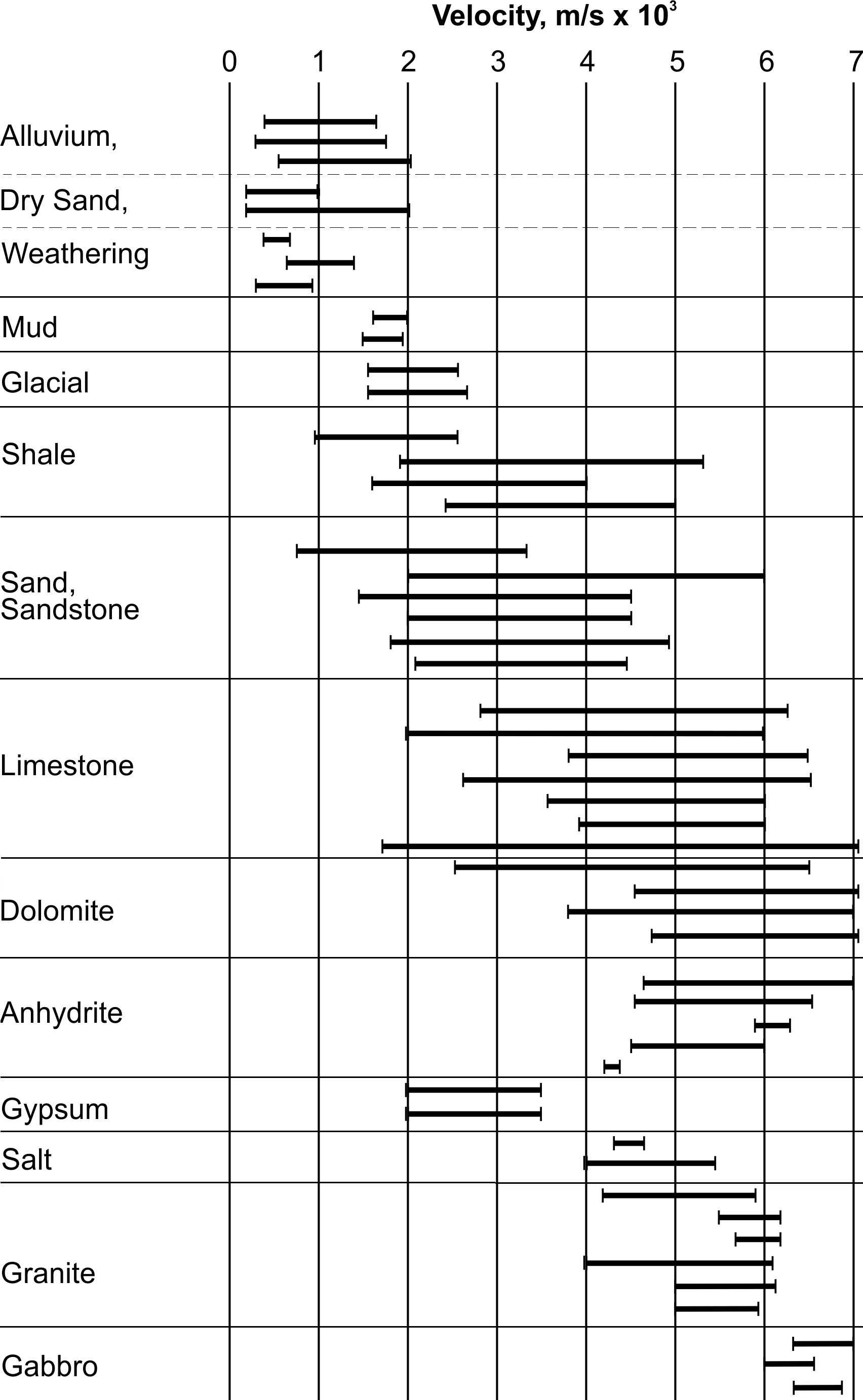
Figure 146. Seismic velocities of different rock types. (Modified from Exploration Seismology, R.E. Sheriff and L.P. Geldart)
The minerals comprising bedrock are almost always electrical insulators. Thus, electrical conduction occurs because of the moisture contained within the pores of the rock or soil. The resistivity of soil or rocks depends on several parameters. These include the clay content, moisture salinity, degree of saturation of the pores, and the number, size, and shape of the interconnecting pores. For soils, the degree of compaction (influencing porosity) is also an important factor. Archie (1942) developed an empirical formulae relating resistivity to porosity, degree of saturation and resistivity of the saturating moisture, shown below.
 (5)
(5)
where 𝝓 is the fractional pore volume (porosity), S is the fraction of the pores containing water, 𝝆w is the resistivity of the water, n is approximately 2, 𝜶 and m are constants with 𝜶 varying between 0.5 and 2.5 and m varying between 1.3 and 2.5.
Porosity determines the amount of water that a rock can contain, and this influences resistivity. However, because resistivity is also influenced by several other factors as described above, the absolute value of porosity can probably not be obtained from resistivity. However, changes in resistivity may possibly be used to indicate changes in porosity, assuming that the other factors influencing resistivity remain constant over the area of interest. In this case, resistivity changes may possibly be used to indicate changes in lithology.
It appears, therefore, that it is not easy to predict lithology from either seismic velocity or resistivity, although rock type is often interpreted from resistivity and seismic velocity data. As discussed above, these methods may be used to map changes in lithology and will be discussed within this context.
Magnetic methods will also be briefly described, since these can be used to estimate the magnetic susceptibility of a rock, which is related to the amount of magnetite it contains. Induced polarization is also described, since this technique is used to locate pyrite and other metallic sulfides.
Some of the methods discussed can be used for investigations to depths of hundreds of meters and beyond. These include seismic reflection and magnetic methods. Seismic reflection methods are used extensively for hydrocarbon exploration surveys. Although the general techniques employed for hydrocarbon exploration are similar to those used for shallower surveys, this web manual concentrates only on techniques applicable to these shallower surveys. It is assumed that the primary depths of concern for this web manual are generally less than 100 m.
Methods
Six different geophysical methods will be discussed. These are listed below along with the observed or derived properties that are measured.
| Method | Observed/Derived Property |
| Seismic Reflection | Layer stratigraphy, and possibly depth |
| Seismic Refraction | Rock velocity, layer depth |
| Time Domain Electromagnetic Methods | Resistivity, layer depth |
| Resistivity Methods | Resistivity, layer depth |
| Magnetic Methods | Magnetic susceptibility, magnetite content |
| Induced Polarization | Metallic sulfides, clay |
Seismic Methods
Two seismic methods will be discussed. These are seismic refraction and seismic reflection. Seismic refraction can be used to obtain vertical and lateral variations in seismic velocity in the shallow subsurface. Seismic reflection can also be used to estimate the velocity and measure the thickness of rock layers, but is more commonly used to map the continuity of reflecting horizons to much greater depths than the seismic refraction method.
Seismic Refraction
Basic Concept: The seismic refraction method can be used to measure rock velocities and the depths to refractors. The method requires a seismic energy source, usually a hammer for depths less than 30 m and black powder seismic guns for depths over 30 m. The seismic waves then penetrate the overburden and refract along the bedrock surface. While they are traveling along this surface, they continually refract seismic waves back to the ground surface. These are then detected by geophones placed on the ground surface. Both compressional waves and shear waves can be used in the seismic refraction method, although compressional waves are most commonly used.
Figure 114b shows the StrataVisor NZ instrument manufactured by Geometrics. This system can record 64 channels of data. In addition, the number of channels can be increased using attached secondary instrumentation. This instrument is used for both seismic refraction and seismic reflection surveys.
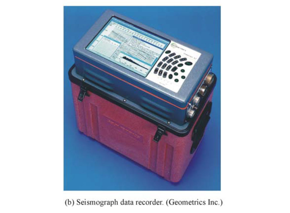
Figure 114b. Seismic Refraction data recorder.
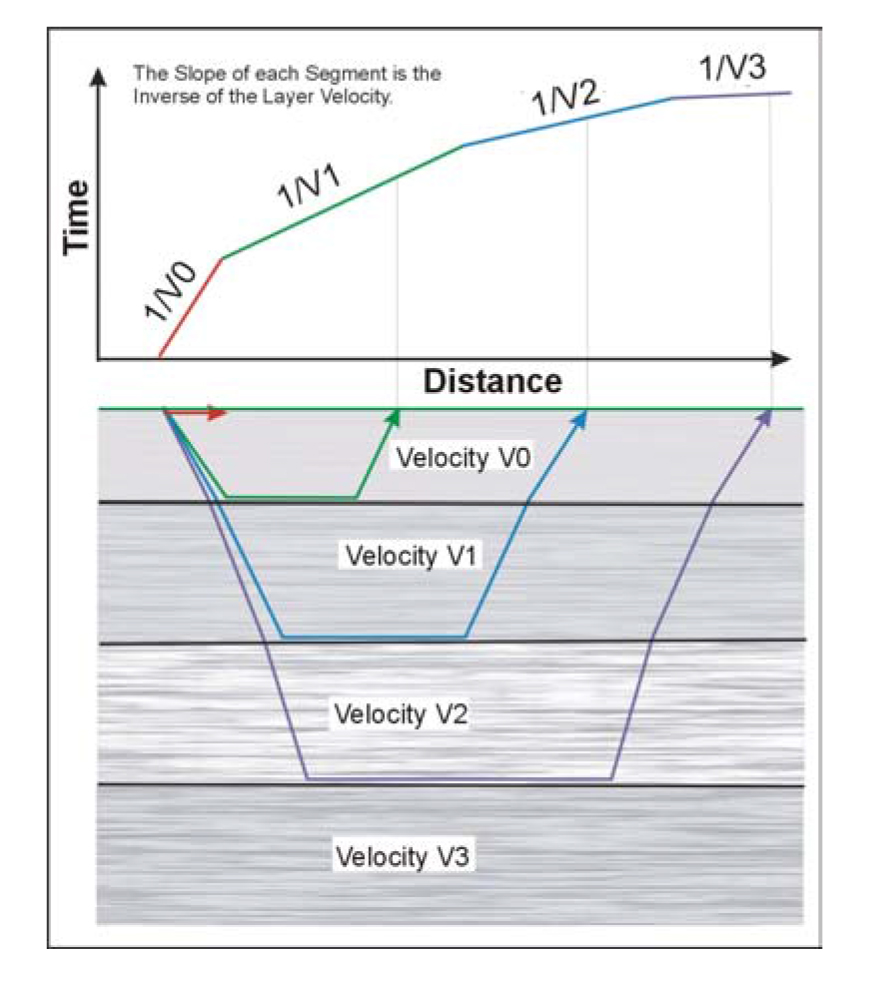
Figure 147. Seismic time-distance graph over four-layer ground.
The main seismic waves and the resulting time distance graph are shown in Figure 114a. This Figure shows the shot locations commonly used in seismic refraction surveys along with the geophone layout. In addition to the shot locations shown, more shots internal to the geophone spread are sometimes used to better map the near surface velocities and stratigraphy.
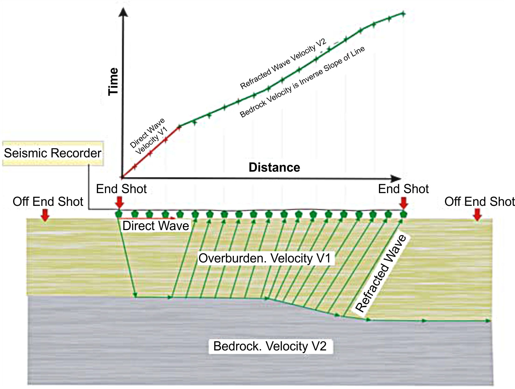
Figure 114a. Seismic Refraction: field set up.
The ray paths and time distance graph over four-layered ground are shown in Figure 147. The inverse of the slopes of the line segments on the time-distance graph provide the velocities of the refractors.
Data Acquisition: The design of a seismic refraction survey requires a good understanding of the expected bedrock and overburden. With this knowledge, velocities can be assigned to these features and a model developed that will show the parameters of the seismic spread best suited for a successful survey. These parameters include the length of the geophone spread, the spacing between the geophones, and the expected first break arrival times at each of the geophones. Knowing the expected first break arrival times is helpful in the field, where field arrival times that correspond fairly well to expected times help to confirm that the spread layout has been appropriately planned, and that the target layers are being imaged. If lateral changes in velocity are required over a wide area, contiguous spreads will be used along traverses crossing the area of interest.
Data Processing: The first step in processing/interpreting refraction seismic data is to pick the arrival times of the earliest seismic signal, called first break picking. A plot is then made showing the arrival times against distance between the shot and geophone. This is called a time-distance graph. An example of such a graph for two-layered ground (overburden and refractor) is shown in Figure 114a and that over four-layered ground is shown in Figure 147. In Figure 114a, the time-distance plot shows the waves arriving at the geophones directly from the shot (Velocity 1). These waves arrive before the refracted waves. The refracted waves arrive ahead of the direct arrivals (Velocity 2). These waves have traveled a sufficient distance along the higher speed refractor (bedrock) to overtake the direct wave arrivals. A similar argument is made for all of the waves shown in Figure 147, where the first arrival waves from each successively faster refractor eventually arrive earlier than the first arrival waves from the slower refractors
Data Interpretation: Several methods of refraction interpretation are used. In recent years, seismic refraction tomography (SRT) has gained popularity and is now the most common method used for interpreting refraction data. The main benefit with SRT is that it allows for obtaining a picture of the velocity distribution in the subsurface highlighting continuous lateral and vertical changes in velocity rather than assuming a layered model.
The SRT technique involves an automated search for the minimum deviation between the measurements made on the ground and the "virtual" measurements of a synthetic model through an iterative computer process. An example of a SRT velocity model is shown in Figure 114c.
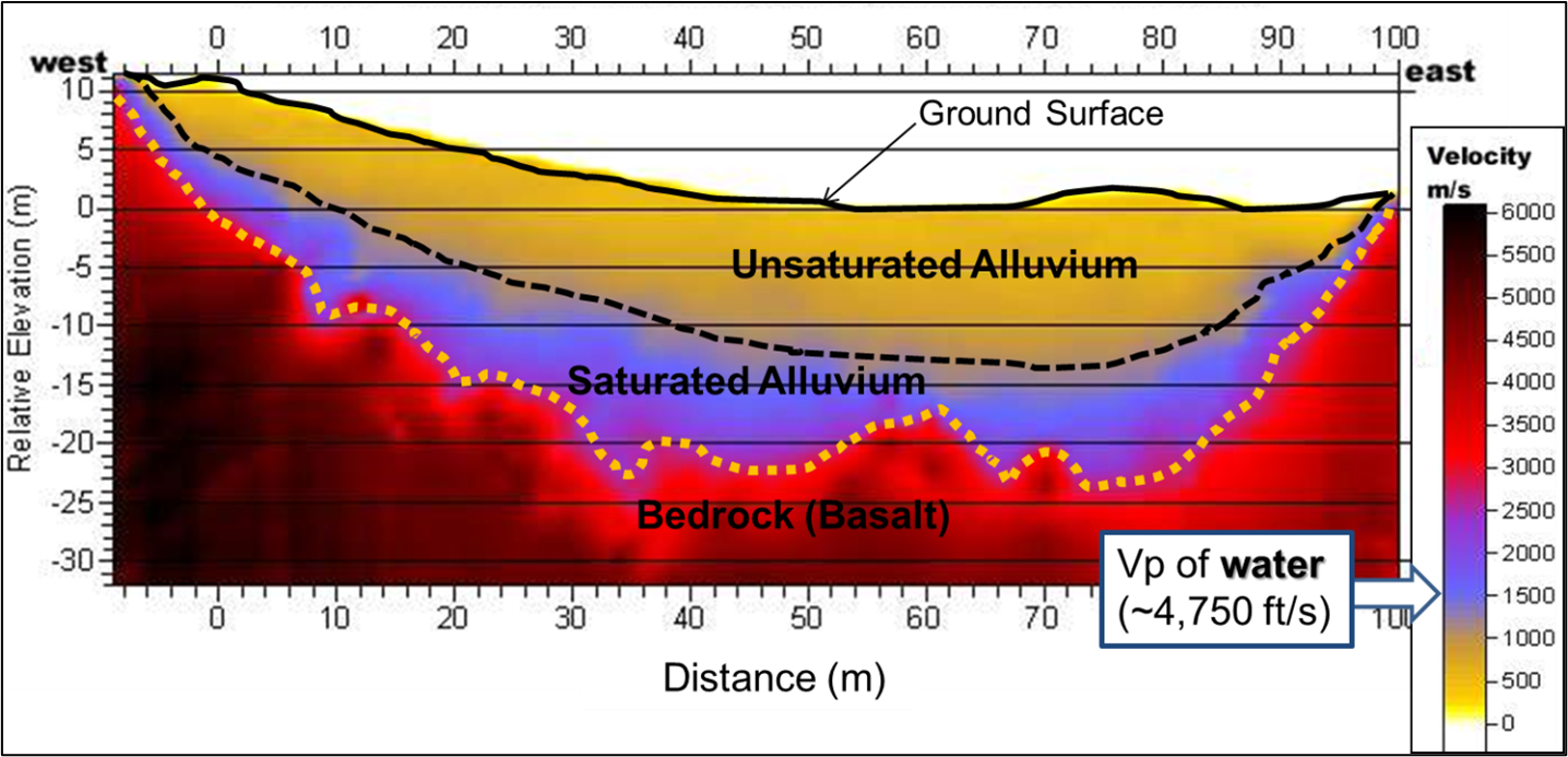
Figure 114c. Bedrock and water table mapping (Image courtesy of USGS).
Another common method is the Generalized Reciprocal Method (GRM) that is described in detail in the Geophysical Methods section. A brief, and simplified, description of the GRM method is presented below. Figure 115 shows the basic rays used for this interpretation.
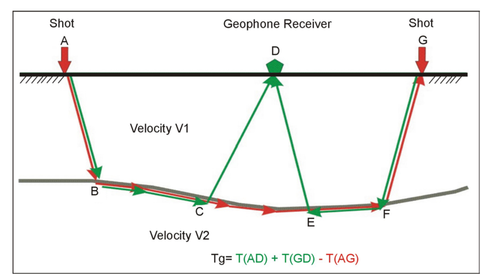
Figure 115. Basic Generalized Reciprocal method interpretation.
The objective is to find the depth to the bedrock under the geophone at D. This is done using the following simple calculations. The travel times from the shots at A and G to the geophone at D are added together (T1). The travel time from the shot at A to the geophone at G is then subtracted from T1. Figure 116 shows the remaining waves after the above calculations have been performed. These are the travel times from C to D added to the travel times from E to D subtracting the travel time from C to E. The sum of these travel times can be shown to be approximately the travel time from the bedrock at H to the geophone at D. Since the velocity of the overburden layer can be found from the time-distance graph, the distance from H to D can be found giving the bedrock depth. This process can be extended to apply to several layers.
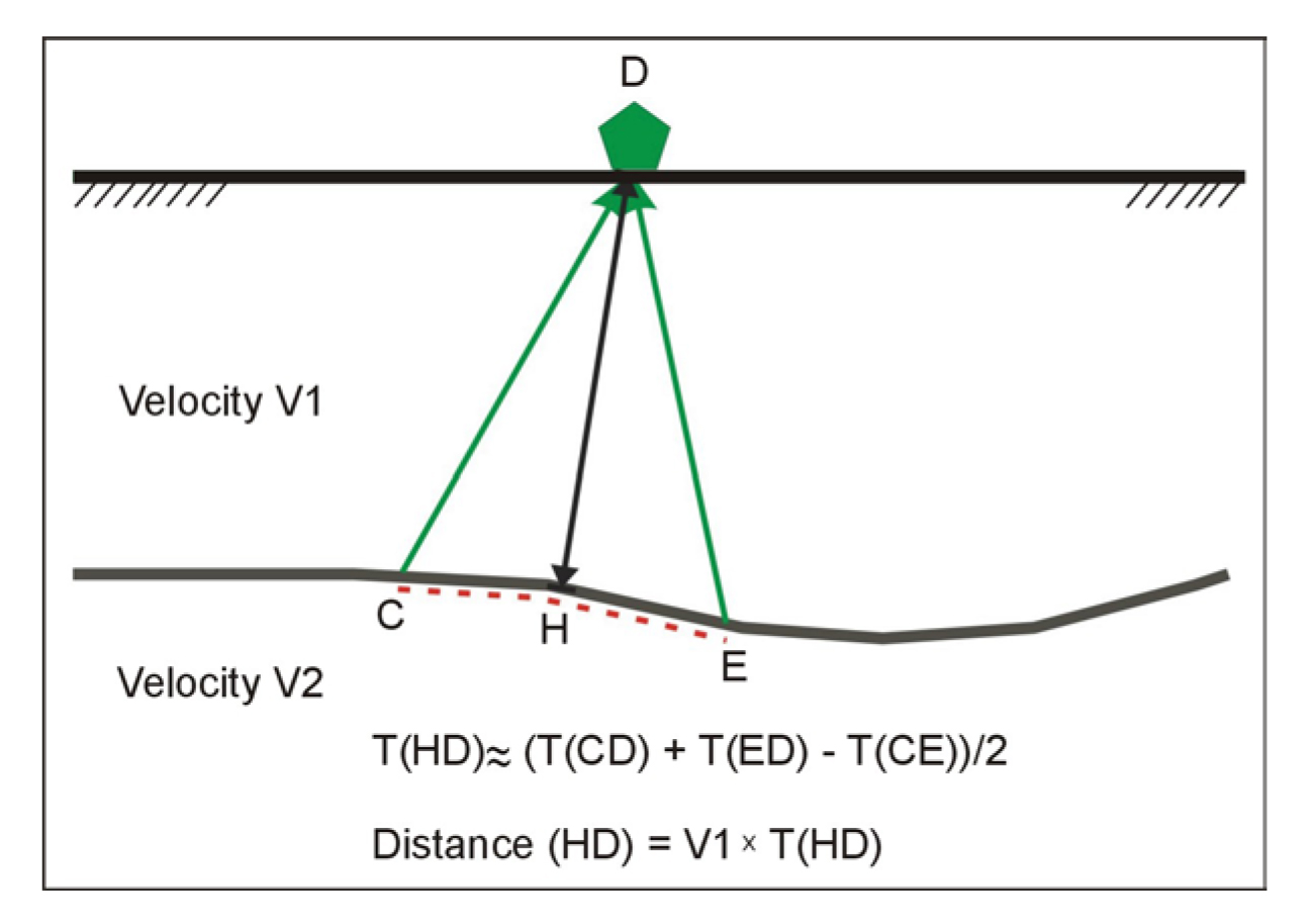
Figure 116. Generalized Reciprocal method interpretation.
Once the velocities of the layers are assigned, these should be interpreted to give appropriate geologic layers. For example, a layer with a velocity of 2,000 m/s suggests a soft rock such as shale, whereas a velocity of 4,000 m/s indicates a hard rock such as limestone. Lateral changes in the velocity of the layers may indicate changes in lithology.
Advantages: Seismic refraction is usually a good method to obtain the velocity of rocks, which one of the criteria for establishing lithology.
Limitations: Probably the most restrictive limitation is that each of the successively deeper refractors must have a higher velocity than the preceding shallower refractor. If this is not the case, errors in depth estimates of the deeper layers can occur, since a lower velocity layer beneath a higher velocity layer will not be observed in the data.
If the water table is in the overburden and close to the bedrock, this may obscure the bedrock arrivals since saturated soils have a higher velocity than unsaturated soils. This may also lower the velocity contrast between the saturated overburden and the bedrock.
Local noise, for example traffic, may obscure the refractions from the bedrock. This can be overcome by using larger impact sources or by repeating the impact at a common shot point several times and stacking the received signals. In addition, since some of the noise travels as airwaves, covering the geophones with sound-absorbing material may also help to dampen the received noise.
Seismic Reflection
Basic Concept: Geological layers can be mapped using the seismic reflection method. This can be done using either a shear wave source or a conventional compressional wave seismic source. One shear wave source is called the Microvib and is illustrated in Figure 8. Compressional wave sources range from a simple hammer and base plate, to black powder and conventional explosive sources, to vibrators. For relatively shallow investigations, a hammer and base plate, weight drop, and black powder sources can be used. The actual depth of investigation depends on the geology and site conditions, but can be 50 m and deeper. For deeper investigations, a small vibrator can be used. Examples are the Microvib (Figure 95) shear wave source and the Minivib source (Figure 148), applicable for depths over 1,000 m.
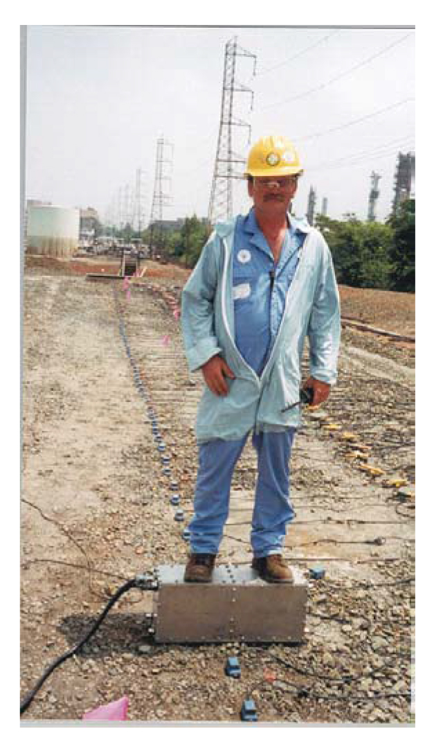
Figure 95. The Microvib shear wave generator. (Bay Geophysical)
Seismic sources, producing either vibrations or impulses can be used for seismic reflection surveys. Special processing techniques are applied to the vibrational sources to make the resulting data compatible with impulse sources.
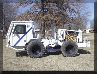
Figure 148. The Minivib seismic source. (Industrial Vehicles, Inc.)
Seismic reflection involves using a surface seismic source to create a seismic wave, which then travels into the subsurface. At interfaces that have an impedance contrast (related to velocity and density), a portion of these waves is reflected back to the ground surface, and a portion is transmitted through the interface. Geophones on the ground surface record these reflections. Figure 118 shows the seismic ray paths for reflections from two layers. The signals at two geophones are illustrated to the right of the ray path diagram. The reflection from the interface between layers 1 and 2 arrives first at geophone 1. A short time after this arrival, the same interface provides a reflection that arrives at geophone 2. Some time later, the reflection from the boundary between layers 2 and 3 arrives at geophone 2.
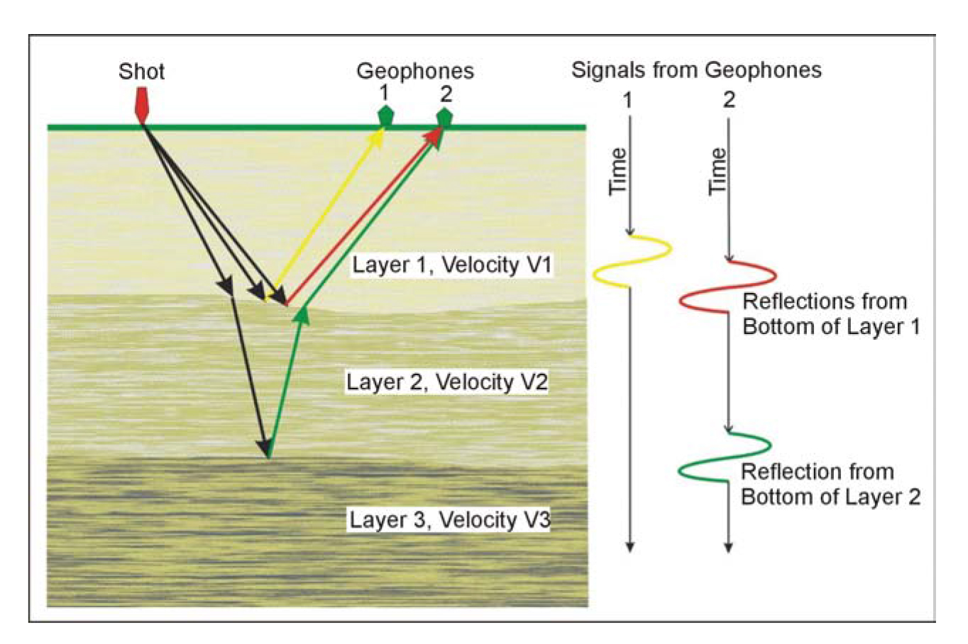
Figure 118. The Seismic Reflection method.
Data Acquisition: In a seismic reflection survey, shots are positioned at regular intervals along the line to be surveyed, and the seismic reflections recorded by a series of geophones placed on the ground surface, called a geophone spread. The number of geophones varies from 12 to 60 or more for non-hydrocarbon seismic surveys. The data are stored in the seismic recorder and transferred to a computer for processing. The spacing between the geophones, the number of geophones used, and the shot spacing have to be determined before the survey begins and depend on the exploration depth and the target resolution required.
Data Processing: If a vibration source is used, such as the Microvib, then special processing techniques have to be applied to make the data compatible with an impulse source.
Many techniques are used to process reflection seismic data including filtering, correcting for velocity effects, and stacking the traces that emanate from a common depth point (CDP, sometimes called common midpoint CMP) on the reflecting surface. The main objective of these techniques is to provide a gather of seismic traces that can be stacked to image each reflection point (CDP) as clearly as possible. The output from processing a line of seismic data is a seismic section showing the reflectors. This section can be presented as CDP location against record time or, when velocities are assigned to the different layers, as CDP against depth.
Data Interpretation: Reflection seismic surveys are usually used for stratigraphic exploration, and a seismic section showing CDP against depth is most appropriate. Such a section should provide an immediate view of the seismic stratigraphy, both vertically and laterally. The relation between the reflector stratigraphy and lithology will need to be constrained using other data such as a well log. This may enable the seismic reflectors to be associated to a particular rock type. Lateral changes in the character of the seismic reflector may indicate changes in the lithology.
Figure 133 presents a seismic reflection section showing several reflectors and interpreted faults. As can be seen, the character of some of the reflectors change across the section. In particular, some of the reflectors are more pronounced and some are less pronounced between the faults. Presumably, at least some of these changes are related to lithological changes.
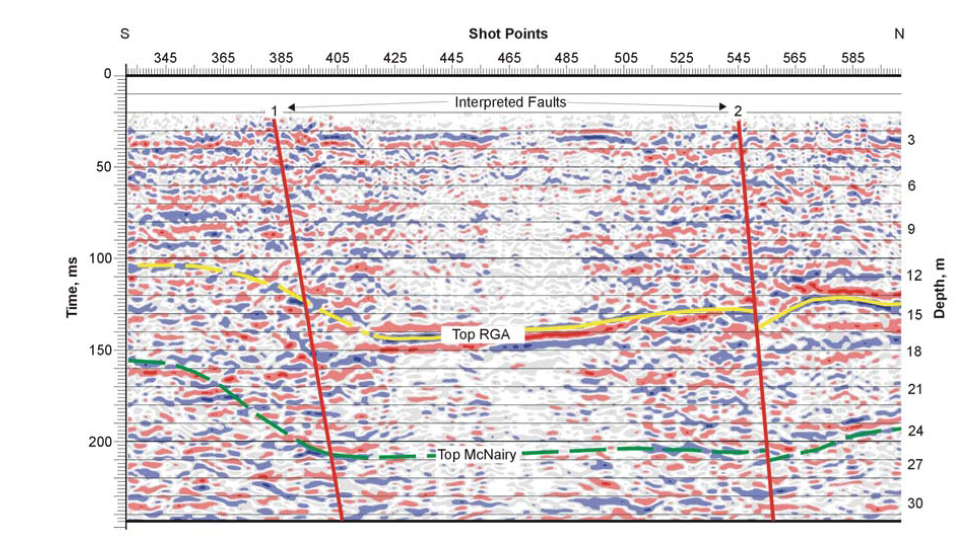
Figure 133. Seismic Reflection section showing faults.
Advantages: The seismic reflection method provides a pictorial section that resembles the subsurface layers. The method is not restricted, as is the seismic refraction method, to a section in which the layer velocities successively increase.
Limitations: The main attribute of the seismic reflection method is that it provides a visual image of the continuity of the reflectors along the surveyed line. Layer velocities are also interpreted but are probably not as reliable as those found using the seismic refraction method. In addition, the method is best suited for investigation depths greater than 10 to 20 m, depending on the geology.
The seismic reflection method is one of the more expensive methods geophysical methods, and requires a significant amount of knowledge to process the data. In addition, any local vibrational noise will reduce the signal-to-noise ratio and make the resulting seismic section less definitive.
Time Domain Electromagnetic Soundings
Basic Concept: Time Domain Electromagnetic soundings (TDEM) are used to obtain the vertical distribution of resistivity. This method is particularly well suited to mapping conductive layers. To a significant degree, this method has now superseded the resistivity sounding method since it requires less work for a given investigation depth and generally provides more precise depth estimates. However, resistivity soundings are still useful for shallow investigations or when resistive targets are sought.
TDEM soundings are an electromagnetic method used to provide the vertical distribution of ground resistivity. The method uses pulses of electromagnetic energy rather than continuously oscillating electromagnetic sources. Figure 120 illustrates the system layout and the current and voltage waveforms.
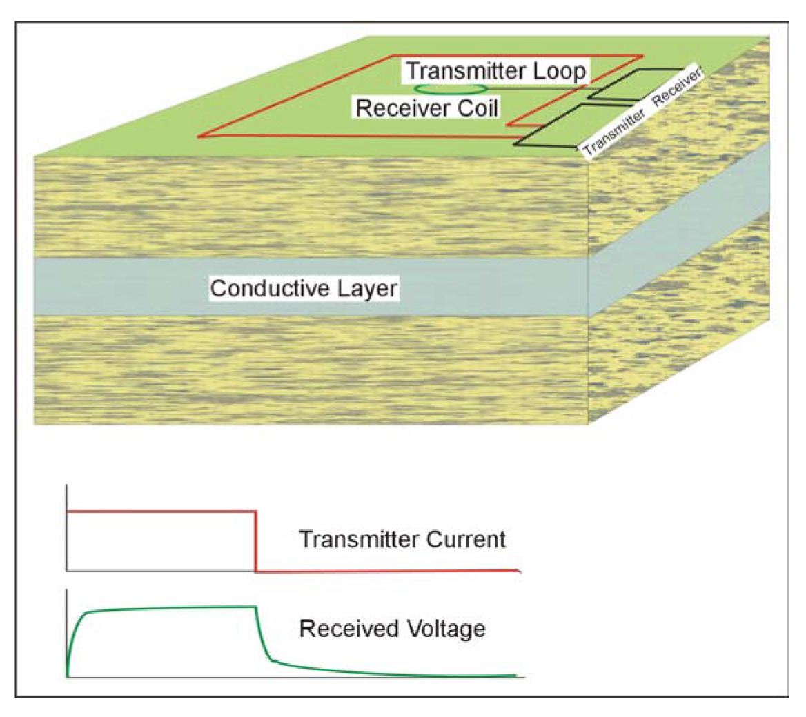
Figure 120. Time Domain Electromagnetic Sounding.
A square loop of wire is laid on the ground surface. The side length of this loop is about half of the desired depth of investigation. A receiver coil is placed in the center of the transmitter loop. Electrical current is passed through the transmitter loop and then quickly turned off. This sudden change in the transmitter current causes secondary currents to be generated in the ground. The currents in conductive layers (shale) decrease more slowly than those in resistive layers. The relation between the time after the current turns off (called delay time in this web manual) and layer depth and conductivity is complex. However, in general, longer decay times correspond to greater depths.
The voltage measured by the receiver coil does not decay instantly to zero when the current is turned off but continues to decay for some time. This decaying voltage is caused by the decaying secondary electrical currents in the ground. The voltage measured by the receiver coil is then converted to resistivity.
A plot is made of the measured resistivity against the delay time, as illustrated in Figure 121. In this graph, the shallow layers are imaged at early decay times and the deeper layers at later decay times.
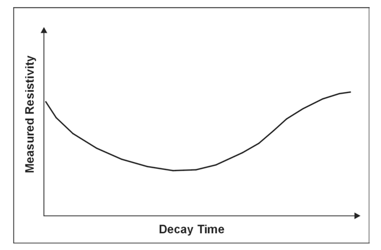
Figure 121. A Time Domain Electromagnetic Sounding curve.
The resistivity sounding curve shown in Figure 121 illustrates the curve that would be obtained over three-layered ground. The near-surface layer is fairly resistive. This is followed by a layer having a much lower resistivity (higher conductivity) and causes the measured resistivity values to decrease. The third layer is again resistive. This method can be used for up to four or five layers.
Data Acquisition: The transmitter loop and receiver coil are set up as described earlier. Switched current is passed through the transmitter loop, and the receiver coil measures the resulting voltage. The switching and measuring procedure is repeated many times allowing the resulting voltages to be stacked and improving the signal-to-noise ratio. Soundings are recorded at different sites until the area of interest has been covered. A sounding curve is plotted for each location showing the measured resistivity against decay time.
Data Processing: Usually the only processing required is the removal of bad data points.
Data Interpretation: The sounding curves are interpreted using computer software to provide a model showing the layer resistivities and thickness. The interpreter inputs a preliminary model into this software program that then calculates the sounding curve for the model. It then adjusts the model and calculates a new sounding curve that better fits the field data. This process is repeated until a satisfactory fit is obtained between the model and the field data. The process is called inversion.
If the TDEM soundings are conducted along a traverse, a section can be drawn showing the variation of resistivity with depth along the section, thus also providing the lateral variations of resistivity. The geologic interpretation then requires that the resistivities be assigned rock types. For example, a shale or clay layer will have a low resistivity, probably less than 30 ohm-m, whereas an impervious limestone may have a resistivity of over 1,000 ohm-m. If a well log is available, rock types can be assigned to the resistivity values with much greater confidence. Lateral changes in resistivity along a particular horizon will possibly indicate changes in lithology.
Advantages: For a given depth of investigation, the method is much more efficient in the field than the resistivity method. The TDEM method is particularly good at defining conductive layers, but less effective at defining resistive layers.
Limitations: Generally, the method is limited to four or five layers. Resistive layers usually have to be fairly thick in order to be resolved, with the thickness increasing with depth. Thin conductive layers can be detected, and, in fact, the method responds to the product of conductivity multiplied by the layer thickness. Thus, thin conductive layers may respond as well as thicker, but less conductive, layers. In these cases, it may not be possible to accurately determine either the thickness or conductivity of the layer.
Metal fences and other above or below ground metal features may prohibit recording interpretable data.
Resistivity
Resistivity methods can be divided into three groups. The first two are resistivity soundings and traverses. The last group combines both resistivity sounding and traverse data to form a resistivity section. Data for this latter group are recorded using relatively recently designed resistivity instruments. Resistivity soundings are useful if the depths and resistivities are needed, although resistivity traverses are now rarely used. This is partially because the ground conductivity can be more easily measured using electromagnetic methods, where no ground contact is required. In addition, resistivity measuring instruments are now available that automatically record data from several different electrode spacings very efficiently, combining traverse and sounding data.
These newer instruments, called automated resistivity systems, use electrodes that are addressable by a central control unit. This means that a large number of electrodes can be placed in the ground prior to starting the survey and connected to the central control unit. The data recording parameters and the electrode array to use are input to the central control unit. Once the electrodes are all connected, the measurements are automatically recorded by the central control unit. Because of the large amount of data obtained with these systems, a more detailed and reliable resistivity interpretation is obtained, making them the preferred instrument for lithology determination.
Resistivity is usually measured using one of the electrode arrays shown in Figure 90. Electrical current is put into the ground using two electrodes, and the resulting voltage is measured using two other electrodes. Since the measured resistivity is a composite of the resistivities of several layers, the correct term is apparent resistivity. In this web manual, the term "measured resistivity" is understood to mean apparent resistivity.
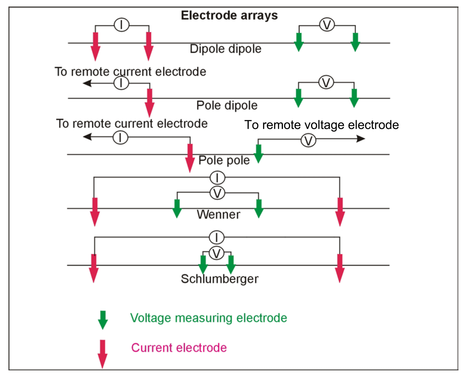
Figure 90. Electrode array used to measure resistivity.
These arrays are used for different types of resistivity surveys. The Schlumberger array is often used for resistivity soundings, as is the Wenner array. The Pole-pole array provides the best signal, but is cumbersome because of the long wires required for the remote electrodes, and it is rarely used. The Dipole-dipole array was originally used mostly by the mining industry for induced polarization surveys. Readings were taken using several different separations of the voltage and current dipoles providing measurements of the variation of resistivity with depth. Long lines of data were recorded requiring many readings. This array has now become common for resistivity surveys using the automated resistivity systems. If more signal (voltage) is needed than can be provided with the Dipole-dipole array, the Pole-dipole array can be used.
Automated Resistivity Systems
Basic Concept: As mentioned above, newer resistivity systems are now available that make taking resistivity measurements much more efficient. Figure 201 shows one such system called the Sting/Swift automated resistivity measuring system.
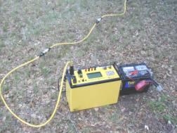
Figure 201. SuperSting R1 IP resistivity meter. (Advanced Geosciences, Inc.)
Data Acquisition: When using these automated resistivity systems, the electrodes for each spread are first placed in the ground and connected to the control unit. This is then programmed with the electrode array desired and other data recording parameters and then instructed to record the data.
Data Processing: Usually the only processing required is the removal of bad data points.
Data Interpretation: Data from the automated resistivity systems are interpreted by inversion software, although much information can be gained visually. An example of the results from such a survey is presented in Figure 149, which shows two high-resistivity zones, each of which contains sand and gravel. The data have been inverted showing the resistivity variation, both laterally and vertically, against depth.
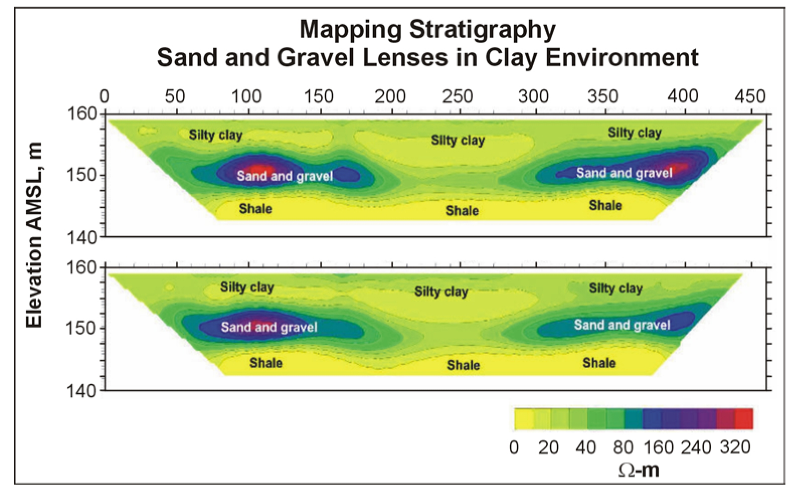
Figure 149. Resistivity data showing stratigraphic changes. (Advanced Geoscience, Inc.)
The low-resistivity areas (less than 20 ohm-m) correspond to clay layers and high-resistivity zones (greater than 100 ohm-m) correspond to sand and gravel lenses. Inasmuch as the change from clay to sand and gravel is clearly observed, and this likely corresponds to a change in grain size, the method has provided some information about changes in lithology.
Advantages: Automated resistivity systems obtain much more data than the simple resistivity systems and therefore are able to give a more detailed interpretation.
Limitations: Since electrodes have to be inserted into the ground, the method is difficult to use in areas where the surface of the ground is hard, such as concrete or asphalt-covered areas. If the ground is dry, water may need to be poured onto the electrodes to improve the electrical contact between the metal electrode and the soil.
If a survey is conducted along a single line, resistivity variations normal to this line are not accounted for in the interpretation. Recording lines parallel to each other, of course, can rectify this problem. In addition, three-dimensional resistivity surveys can now be recorded and interpreted.
Magnetic
Basic Concept: Magnetic methods can be used to estimate the magnetic susceptibility of rock formations, which is related to the amount of magnetite that the formations contain. To the extent that this is mapping mineral content, it can be considered as mapping one parameter related to lithology.
Magnetic data can be recorded using ground or airborne surveys. If large areas are to be covered, airborne surveys may be appropriate. Many considerations need to be evaluated before making a decision whether to use a ground or airborne survey, the most important being the size of the area to be surveyed. Other considerations include the density of data required, the comparative costs, and the expected depth of the target. Only ground surveys are discussed in this section of the website, since the theory of the method and interpretation are similar for both types of surveys.
Rock layers often contain small amounts of magnetite. This magnetite produces a secondary magnetic field that is superimposed on, and distorts, the Earth's magnetic field. Measurements of the magnetic field strength made on the ground surface can be used to determine the depth of the layer containing the magnetite and estimate its magnetic susceptibility. Estimating the susceptibility can only be done approximately, and only an estimate of the amount of magnetite can be given. However, lateral or vertical changes in susceptibility may be able to be used to assess relative magnetite content changes. The magnetic method is not well suited for interpretation of several successively deeper layers containing magnetite, since the magnetic anomaly from the shallowest layer dominates the measured magnetic field.
Several instruments are available for recording magnetic data, one of which is shown in Figure 209. This instrument is also equipped with a GPS system allowing its location to be recorded at all times.
Data Acquisition: Magnetic surveys are conducted by recording data along a traverse crossing the area of interest. Data are normally recorded in time mode, usually at several readings per second. Positioning with the magnetometer illustrated in Figure 209 is with the GPS system. If GPS is not used, other methods are required to position the data.
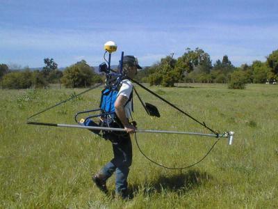
Figure 209. Cesium magnetometer with GPS. (Geometrics, Inc.)
Because the magnitude of the Earth's magnetic field continuously changes in time, a base station is often set up to record these changes. Since these changes usually have a daily cycle, they are called diurnal effects. This station has to be time synchronized with the magnetometer recording the spatial data. The effect of these magnetic variations can then be removed from the field data during processing provided the variations are not too severe. However, if the diurnal magnetic changes become significant, the survey should be stopped.
Data Processing: The magnetic data needs to have the diurnal drift removed, and the data spatial coordinates will have to be assigned. This can be done by obtaining the positions of the ends of each of the lines and using interpolation to assign coordinates to the other data points. However, magnetometers are now available with GPS allowing coordinates to be assigned to the data as they are being recorded (see Figure 209). Various filtering routines can be applied to remove noise spikes and apply some smoothing if needed.
Data Interpretation: The kind of anomaly expected over a magnetite-rich zone is illustrated in Figure 150. Because the direction of the Earth's magnetic field is not vertical (except at the magnetic poles), the anomaly has a positive and negative component and is not symmetrical about the source of the magnetite, which can make the interpretation of the source of the magnetic anomaly difficult. To make interpretation easier, the field strength data can be processed to produce a function that peaks over the top of the source. This is called the Analytic Signal, and is the sum of all of the spatial gradients of the magnetic field strength data. The width of the Analytic Signal at half of its amplitude is related to the depth to the magnetic source, and the amplitude of the Analytic Signal is related to the susceptibility of the magnetite source.
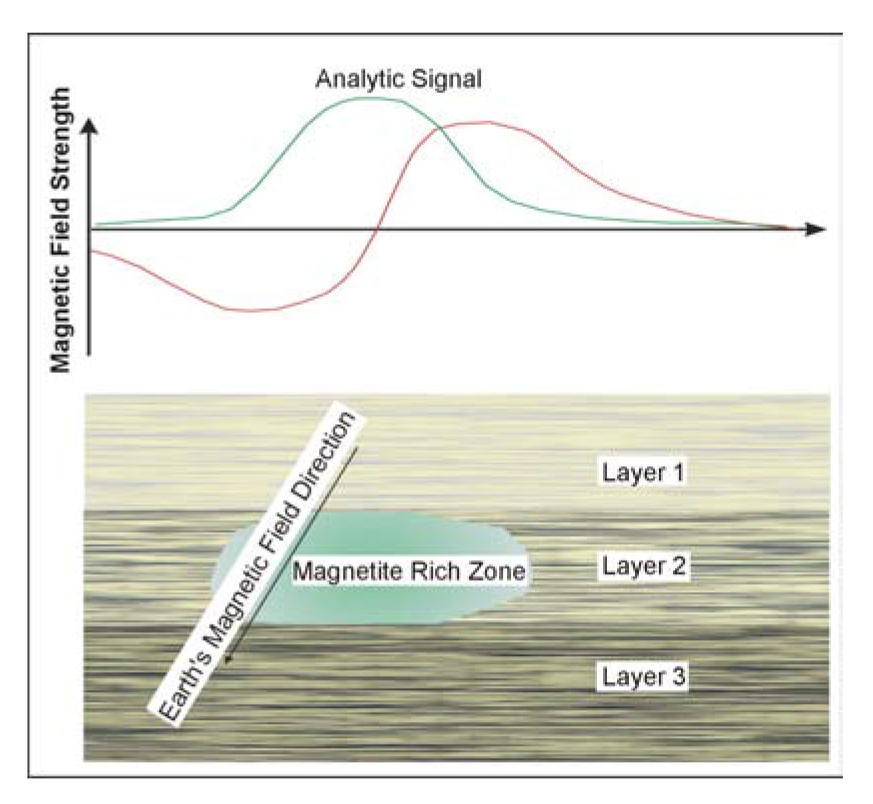
Figure 150. Magnetic anomaly over a magnetite rich zone.
Using the Analytic Signal data (or the magnetic field strength data), estimates can be made of the susceptibility of the magnetite source, which is related to the amount of magnetite in the rocks. The depth to the source can also be calculated. It may be possible using this method to map variations in magnetic susceptibility, which may indicate lithological changes.
Advantages: Magnetic data is relatively simple and efficient to record in the field.
Limitations: Since the source of the magnetic anomalies is a zone of magnetite whose edges are probably not well defined, depth calculations of its depth may have significant errors, since the calculations are based on well-defined source shapes.
If the diurnal variations in the Earth's magnetic field are large, then data recording should be stopped until the diurnal changes diminish. If areas of magnetite are in successively deeper layers, probably only the first layer will be recognized.
Induced Polarization
Basic Concept: Induced Polarization (IP) is commonly used in the mining industry to locate metallic sulfides such as pyrite, chalcopyrite, and other metallic minerals. It is discussed here only because, like the magnetic method, it provides data on the distribution of metallic minerals and could be regarded as mapping changes in lithology. Induced Polarization anomalies are found over metallic sulfides, graphite zones, and some clays.
Induced Polarization is an electrical method that measures the change in the measured resistivity of the ground with frequency. Numerous electrode arrays can be used to measure IP data, several of which are illustrated in Figure 90.
Figure 90. Electrode arrays used to measure resistivity.
For this section of the website, the dipole-dipole array is used to illustrate the waveforms. This is probably the most commonly used array for measuring Induced Polarization. Two methods are used to obtain IP data: time domain and frequency domain. In time domain, a constant current is passed into the ground using two of the four electrodes. This current is then rapidly switched off. During this off time, the remaining two electrodes measure the resulting voltage. If an IP effect is present, the voltage across these electrodes will not suddenly return to zero as the current is turned off, but will decay to zero over a period of time, usually within a few seconds, as illustrated in Figure 110. Simple IP measurements usually integrate the IP voltage over a specified time period, say T1 and T2 providing a single number that is a measure of the IP response. However, if a more detailed analysis is needed, the full voltage and current waveforms are recorded. The units used to measure the IP effect, called chargeability, are mV/V. Using the Fourier transform to convert the data to frequency domain, these data can then be converted to the variation of IP response with frequency, called Spectral IP (SIP). In frequency domain, the IP effect is measured at different current waveform frequencies. If more than two frequencies are used, SIP data are recorded.
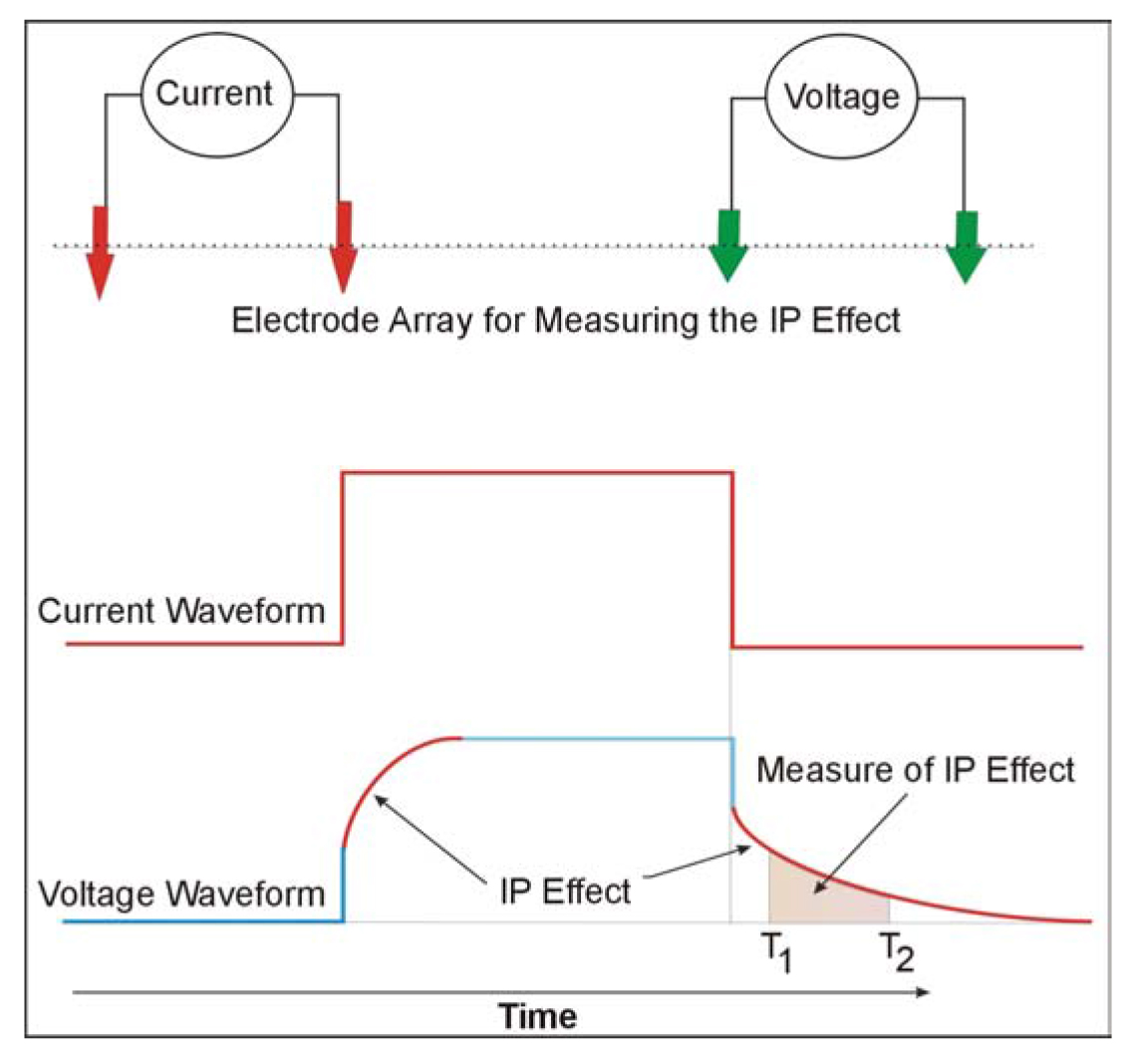
Figure 110. Induced Polarization waveform.
Induced Polarization surveys require electrodes, a data recorder, current transmitter, and a power source for the transmitter. An example of an IP data recorder is shown in Figure 151.
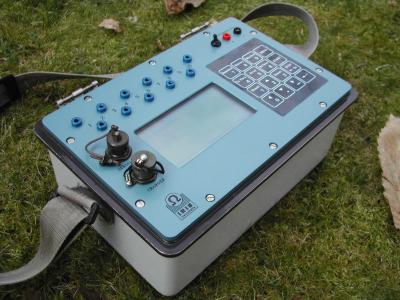
Figure 151. Induced Polarization instrument. (IRIS Instruments)
This particular instrument can record up to 10 channels of data simultaneously. It can also be configured with the automated data recording instrument systems, making data recording efficient.
Data Acquisition: Induced Polarization surveys are conducted much like resistivity surveys. Readings are taken at discrete stations to form lines of data crossing the area of interest. In frequency domain, the variation of IP response with frequency is obtained. In the time domain, if the current and voltage waveforms have been digitally recorded and a Fourier analysis performed, the variation of resistivity with frequency is measured producing SIP data. SIP data provide more interpretable information than the simple IP measure discussed above; however, this is still being researched and is rarely used as a production method. SIP data may be able to distinguish between the different minerals (metallic minerals, graphite, and clay) that produce IP anomalies. However, if the goal is to simply map the occurrence of metallic minerals, spectral IP methods are probably not required.
Data Processing: When recording IP data, resistivity data are also recorded. Both the resistivity and IP data are usually plotted in section form called a pseudosection. With this presentation, data from the smaller electrode separations are plotted near the top of the pseudosection (ground surface), and data from the largest electrode separations are plotted at the bottom of the pseudosection, thus simulating a plot showing resistivity and IP against depth for all values along the traverse. A typical chargeability pseudosection is shown in Figure 152. The horizontal dimension is distance, and the vertical dimension is related to the electrode spacings used to take the measurements. Although these data are from a fairly shallow survey using small electrode spacings, it does illustrate the method, presentation techniques, and the interpretation. Surveys to much greater depths can be performed using larger electrode spacings.
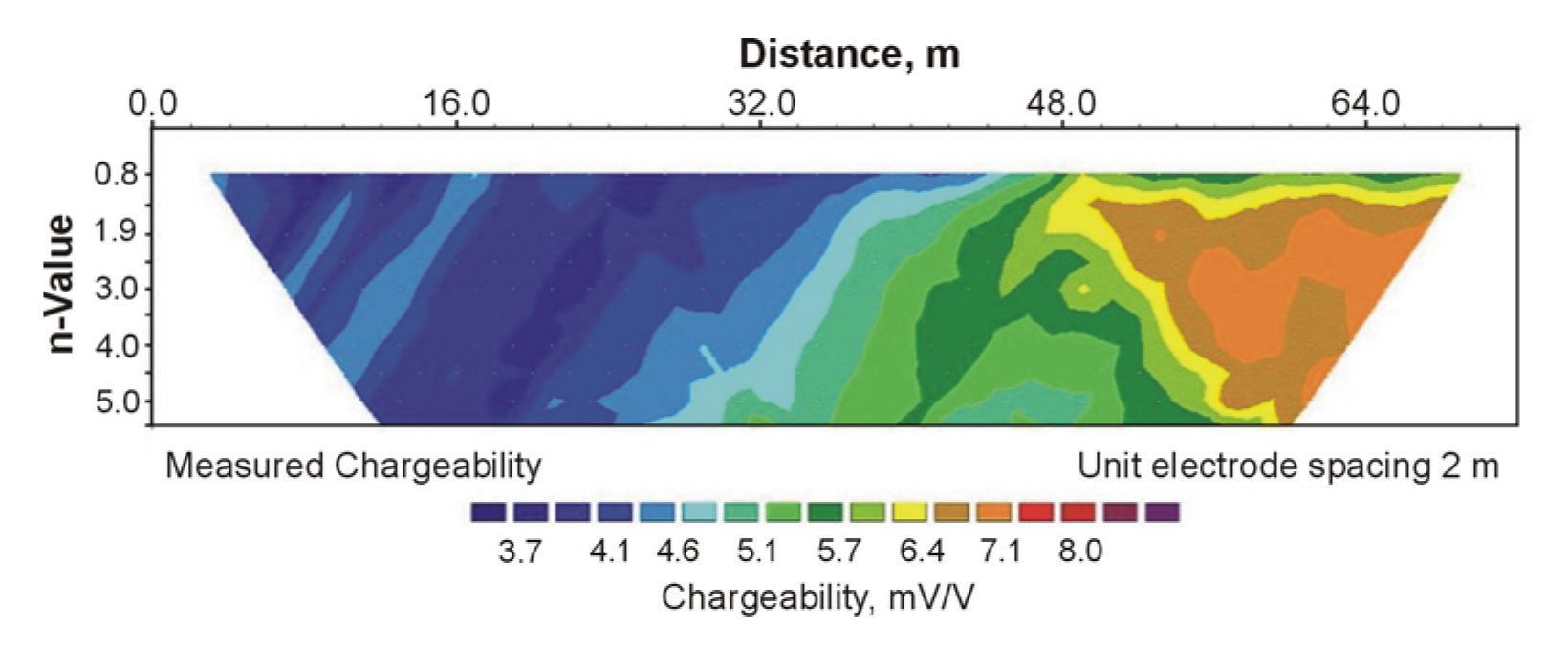
Figure 152. Chargeability pseudosection. (Terraplus, Inc.)
The corresponding resistivity pseudosection is shown in Figure 153.
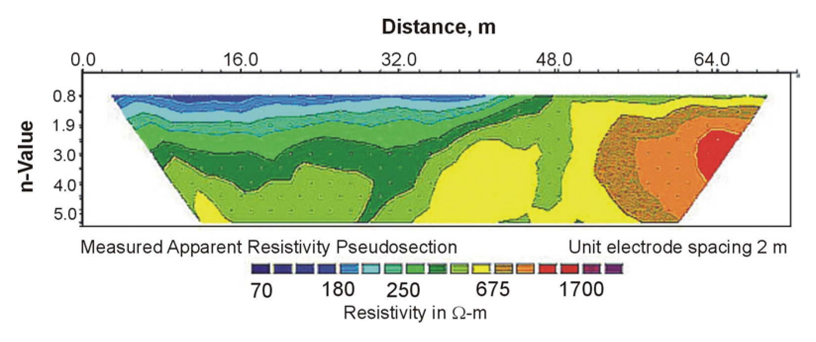
Figure 153. Measured (apparent) resistivity pseudosection. (Terraplus, Inc.)
Data Interpretation: The pseudosection data are usually interpreted by using inversion techniques, where initial model estimates are input to the program, which then calculates the pseudosection resulting from this model. It then determines the degree of fit of the calculated pseudosection with the field data, modifies the model accordingly, and a new pseudosection is then calculated. This process is repeated until the model provides a pseudosection that gives a good fit to the field data.
Figure 154 shows the interpretation of the data presented in Figure 152. In this profile the elevation of the ground surface has also been incorporated into the interpretation.
Since induced polarization phenomena also occur when clays are present in the subsurface, the method can possibly be used to estimate clay content. The survey techniques, processing, and interpretation are similar to those described above for metallic mineral detection.
Although IP anomalies are frequently observed over clays, and reports of its use to find clays are common, no published relationship was found showing a correlation between the magnitude of the IP response and the amount of clay.
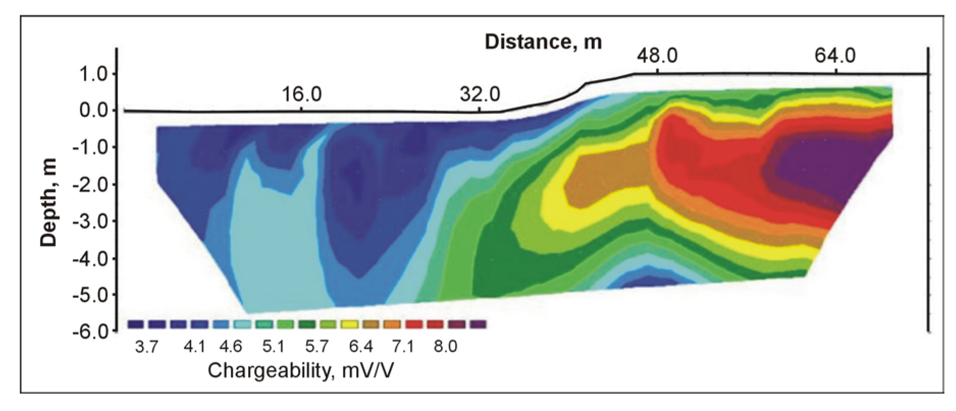
Figure 154. Interpreted Induced Polarization data shown in Figure 152.
Advantages: IP measures the variation of resistivity with frequency and provides a unique interpretation showing polarizable material such as clays, graphite and metallic minerals.
Limitations: The induced polarization method, like the resistivity method, requires electrodes to be inserted into the ground. However, with the IP method, the polarization signals can be quite small, and it is important to put as much current into the ground as possible to increase the measured signals. If the ground surface is hard or dry, it may be difficult, not only to get the electrodes in the ground, but also to put electrical current in the ground. This can usually be solved by pouring water on the electrodes, thereby improving the electrical contact between the electrode and the surrounding soil.
Borehole Gamma Logs (Natural Gamma or Gamma Ray)
The gamma log (also known as natural gamma or gamma ray log) provides a measurement recorded in counts per second (CPS) that is proportional to the natural radioactivity of the formation. This log is used principally for lithologic identification and stratigraphic correlation. Because measured counts are proportional to the quantity of clay minerals present, the gamma log is an excellent indicator of clay layers, including swelling clays.
Basic Concept: Gamma radiation is measured, in counts per second, with scintillation NaCI detectors. The gamma-emitting radioisotopes that naturally occur in geologic materials are Potassium40 and nuclides in the Uranium238 and Thorium232 decay series. Potassium40 occurs with all potassium minerals, including potassium feldspars. Uranium238 is typically associated with dark shales and uranium mineralization. Thorium232 is typically associated with biotite, sphene, zircon and other heavy minerals. Natural radioisotopes occur in exchange ions, which are attached to the clay particles.
Data Acquisition: To record a gamma log, the probe is lowered slowly into a borehole, as depth is precisely recorded with regard to the data-conducting wireline. As the probe proceeds up or downhole, CPS values are recorded at intervals, typically 0.3 cm, and plotted and displayed in real-time (Figure 155). All data is recorded directly to a computer hard-drive, and the data files can be easily transferred via LAN, internet, floppy disk, or CD-ROM.
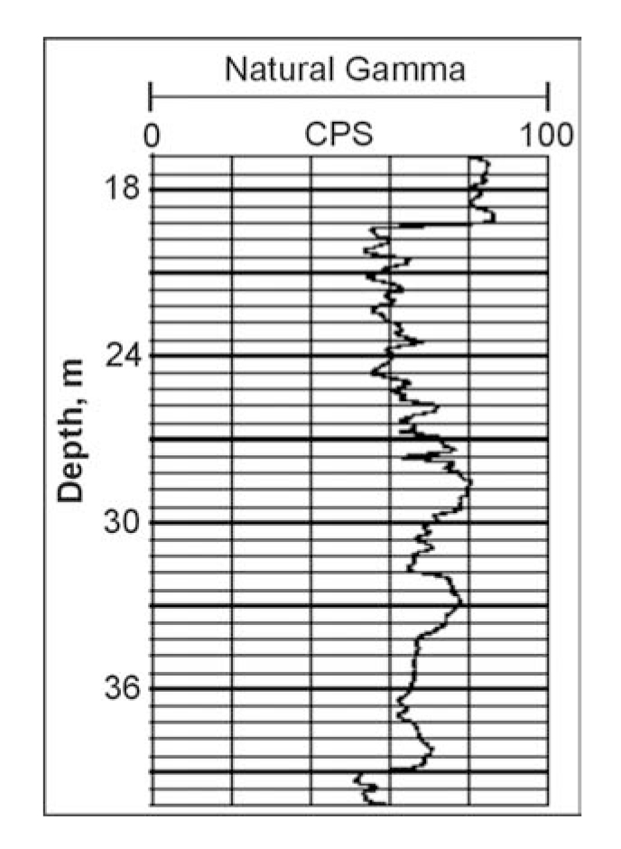
Figure 155. Example of gamma CPS vs. depth. (Layne Christensen, Colog.)
Data Processing: Gamma logs require minimal processing. Plots of CPS vs. depth can be created with raw values or may be filtered slightly to reduce statistical noise.
Data Interpretation: The usual interpretation of the gamma log, for hydrogeology applications, is that measured counts are proportional to the quantity of clay minerals present. This assumes that the natural radioisotopes of potassium, uranium, and thorium occur in exchange ions, which are attached to the clay particles. Thus, the correlation is between gamma counts and the cation exchange capacity (CEC). Usually, gamma logs show an inverse linear correlation between gamma counts and the average grain size (higher counts indicate smaller grain size, lower counts indicate larger grain size). With this simple correlation, depth and extent of layers containing clay particles can be established.
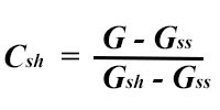
The assumption of a linear relationship between the clay mineral fraction in measured gamma activity can be used to produce a shale fraction calibration for a gamma log in the form:
 (6)
(6)
Where Csh is the shale volume fraction, G is the measured gamma activity; Gss is the gamma activity in clean sandstone or limestone; Gsh is the gamma activity measured in shale.
Advantages: The gamma log provides information about the subsurface lithology with very little processing. Interpretation is simple and acquisition is rapid. Natural gamma rays travel through casing and pipe materials, such as PVC and steel. Thus, logs may be recorded within existing holes, including injection, extraction, or monitoring wells, cross-hole sonic tubes, or other borings that have been prepared for other reasons.
Limitations: This relation can become invalid if there are radioisotopes in the mineral grains themselves (immature sandstones or arkose), and if there are differences in the CEC of clay minerals in different parts of the formation. Both of these situations are possible in many environments. The former situation would most likely occur in basal conglomerates composed of granitic debris, and the latter where clay occurs as a primary sediment in shale and another as an authigenic mineral deposited in pore spaces during diagenesis. Gamma logs should be included in a suite of logs that can provide an array of subsurface information. Specific core samples may still be recovered for lab analysis.