The groundwater surface lies at depths ranging from the ground surface to many hundreds of feet. The exact configuration of this surface depends on the geology of the area, topography, and precipitation. In sedimentary areas, the configuration depends on the type of sediments and their grain size. In hard-rock areas, the groundwater surface may exist in the alluvium above the bedrock. If this is not the case, then groundwater may exist in fractures within the rocks, and a well-defined water table may not exist.

The groundwater surface is usually related to the topographic surface, although with smaller elevation changes. Thus the depth to the water table on top of a hill is usually greater than the depth in a valley. Streams and lakes occur where the water table reaches the topographic surface. Figure 162a shows several important features about groundwater and the water table.

If the bedrock is impervious, such as granite and other igneous and/or metamorphic rocks, groundwater can rest in hollows on top of the bedrock, as is illustrated in Figure 162b. The situation shown in Figure 162b is much less common than that illustrated in Figure 162a.

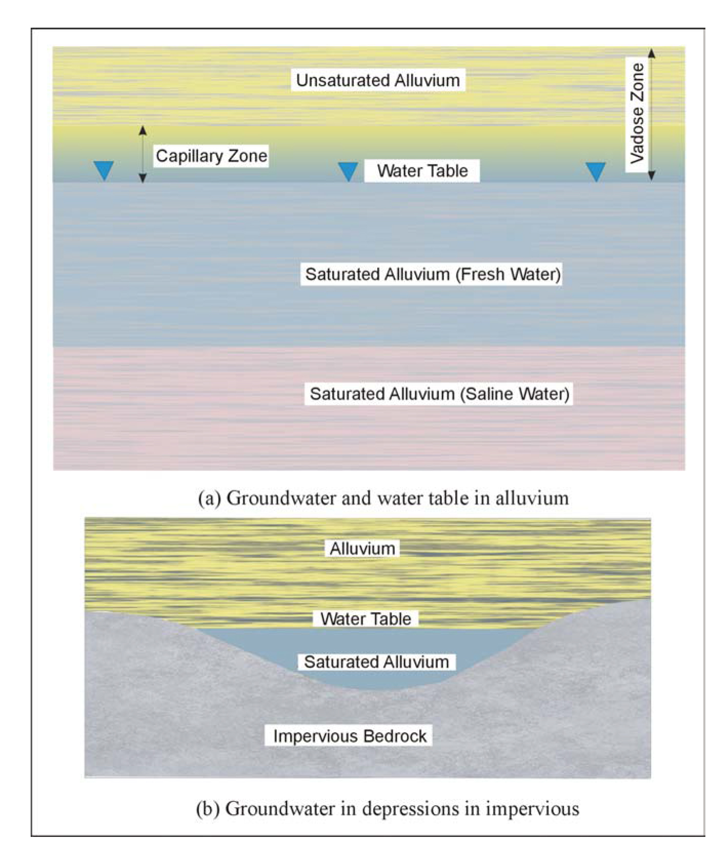
Figure 162. Two common groundwater occurrences.

Groundwater occurs in aquifers, which can be classified as unconfined or confined. In an unconfined aquifer, the water only partially fills the aquifer, and the upper surface is free to rise and decline. Unconfined aquifers are also known as water table aquifers. In a confined aquifer, water completely fills the aquifer, which is overlain by a confining bed, called an aquitard. Aquifers can also be perched, in which an aquitard restricts the downward movement of the water.

Geophysical methods are most applicable to mapping the surface of the water table aquifer, although saturated fracture zones can also be detected. Perched aquifers will probably be difficult to detect because the contrast in physical properties with the surrounding rocks will probably be small. Therefore, the following discussions refer to groundwater and the water table in alluvial geology. Figure 162a shows unsaturated alluvium that transitions into saturated alluvium at depth. The transitional nature of the change from unsaturated to saturated alluvium is caused by capillary action, which draws water from the saturated zone into the unsaturated zone. The height of the capillary zone depends significantly on the grain size of the alluvium. If the alluvium were mostly cobbles, which could be classified as very large grain sizes, there would be very little capillary action, and the capillary zone would be very small. In this case, the water table is well defined and is the best case for detection by geophysical means.

If, however, the alluvium is fine grained, then the height of the capillary zone can be quite large. In this case, the water table is very poorly defined, making its surface more difficult to map. Eventually, at some depth, the fresh water usually becomes more saline. The thickness of the freshwater layer varies considerably from a few meters to many hundreds of meters.

The physical properties that may be used to map the top of the water table are resistivity and seismic velocity. Ground Penetrating Radar (GPR) may also be useful for some locations. One new method that has been investigated is called Nuclear Magnetization Resonance (NMR), which will be briefly discussed along with a method called the Electroseismic method that is said to provide hydraulic conductivity values.

As discussed previously, when there is a large capillary zone, the measurable physical properties change gradually from the unsaturated zone to the saturated zone. Thus, resistivity changes gradually from being resistive to conductive; this is the same for seismic velocity.

Methods: Groundwater Surface

Resistivity Soundings

Basic Concept: Mapping the groundwater surface will usually require sounding methods. Resistivity, or conductivity, soundings may be appropriate since there may be a significant resistivity contrast between the unsaturated soil and the saturated alluvium. Generally, the contrast will be greater for coarse-grained alluvium than for fine-grained alluvium. This is because fine-grained unsaturated alluvium can hold and retain more moisture than coarse-grained alluvium.

Ground resistivity is measured using four electrodes inserted into the ground. Two of the electrodes are used to pass electrical current into the ground, and the other two are used to measure the resulting voltage. A number of different electrode arrays are used and are illustrated in Figure 90. The Schlumberger array is often used for resistivity soundings, as is the Wenner array. The Pole-pole array provides the best signal but is cumbersome because of the long wires required for the remote electrodes, and it is rarely used. The Dipole-dipole array was originally used mostly by the mining industry for induced polarization surveys. Readings were taken using several different separations of the voltage and current dipoles providing measurements of the variation of resistivity with depth. Long lines of data were recorded requiring many readings. This array has now become common for resistivity surveys using automated resistivity systems. If more signal (voltage) is needed than can be provided with the Dipole-dipole array, the Pole-dipole array can be used.

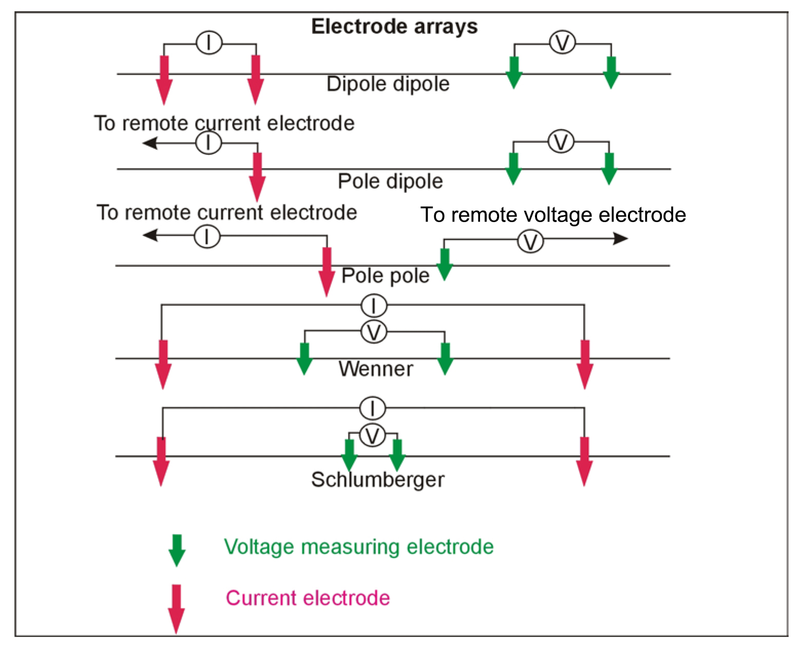
Figure 90. Electrode arrays used to measure resistivity.

Resistivity data can be recorded using one electrode spacing and taking readings along a traverse or by taking readings using a number of different electrode spacings while keeping the location of the center of the array fixed. When the center of the array remains fixed, it is called a resistivity sounding. To map water table depths only, resistivity soundings are likely to be used since resistivity traverses would only provide lateral changes in resistivity and not depths. However, for detailed surveys, automated resistivity systems, which record data using many electrode spacings, may be used. These are described later in this section.

Figure 91 shows resistivity measured with the Schlumberger electrode array (Figure 91a) and the sounding curve (Figure 91b) over an unsaturated resistive near-surface layer and conductive saturated layer. In this Figure, the current is injected into the ground using the two outer electrodes, and the resulting voltage is measured using the two inner electrodes. Figure 91b is a plot of the measured resistivities against the current electrode spacing. As Figure 91b shows, at small electrode spacings the measured resistivity approaches that of the near-surface unsaturated layer, whereas at large electrode spacings, the measured resistivity approaches that of the saturated layer.

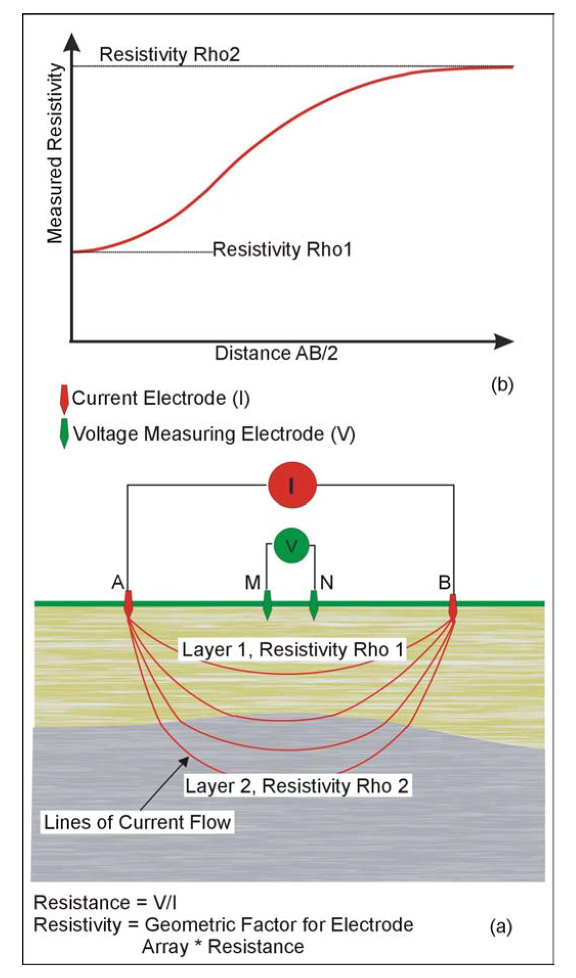
Figure 91. Electrode array for (a) measuring the resistivity of the ground, and (b) a resistivity sounding curve.

Since the measured resistivity is usually a composite of the resistivity of several layers, the term "Apparent Resistivity" is usually used. In this website, the term Apparent Resistivity is usually referred to simply as "measured resistivity." Apparent Resistivity is calculated using the equations shown at the bottom of Figure 91.

To conduct a resistivity sounding, resistivity data are recorded at a number of electrode spacings, since electrode spacing determines the depth of investigation. These resistivity values are then plotted against the electrode spacing used to obtain the measurements to produce a resistivity sounding curve, illustrated in Figure 91b. Figure 163 shows an instrument used to measure the resistivity of the ground.

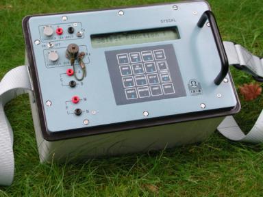
Figure 163. Resistivity instrument. (IRIS Instruments)

Data Acquisition: Resistivity soundings are conducted by initially planting the electrodes in the ground using a fairly small electrode spacing (a few meters) and taking a reading. This process is repeated using larger electrode spacings while keeping the center of the array fixed until the desired layer is imaged. It is usually advisable to plot the resistivity sounding curve in the field in order to evaluate the data. Where the groundwater surface is desired, data will be recorded from successively larger electrode spacings until the measured resistivity values are clearly decreasing, showing that a conductive layer has been imaged.

Data Processing: Bad data points need to be removed after which the measured resistivity data are plotted against electrode spacing, and a preliminary interpretation made.

Data Interpretation: The resistivity sounding data and the model are input to a computer program that inverts the data to produce a layer depth and resistivity model whose sounding curve matches that of the field data. Inversion is a process whereby the computer program calculates the sounding curve from the model and then compares this with the field data. It appropriately modifies the model and calculates another sounding curve, repeating this process until the sounding curve from the model matches that from the field data.

Advantages: Resistivity soundings are fairly easy to record and are an effective sounding technique down to depths of 50 meters, depending on the geology. A sounding curve can be plotted in the field and can be visually interpreted to provide very approximate estimates of the subsurface resistivities and depths.

Limitations: Resistivity soundings require electrodes to be placed in the ground. If the ground surface is hard, placing the electrodes may be difficult. The interpretation of resistivity soundings assumes that the geological layers under the sounding site are horizontal and homogeneous, with no lateral changes in resistivity. If these conditions are not met, the interpretation will not be correct. Errors in the field data can occur if soundings are recorded close to grounded metallic features such as fences or parallel subsurface utilities.

Generally, the separation between the current electrodes will need to reach a maximum of about three times the investigation depth. Thus, if the bedrock is 15 m deep, the current electrodes will need to be spaced up to 46 m apart.

Automated Resistivity Systems

Basic Concept: Resistivity systems are available that make taking resistivity measurements much more efficient, automatically taking many measurements at different electrode spacings along a traverse. These systems are able to build a comprehensive picture of the subsurface, combining both lateral and vertical variations in resistivity. Figure 201 shows an example of automated resistivity measuring system called the Sting/Swift system.

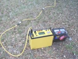
Figure 201. SuperSting R8 IP resistivity meter. (Advanced Geosciences, Inc.)

Data Acquisition: With these systems, many electrodes are planted and connected to the central recorder before taking any data. When this is done, the recording parameters for the survey are entered into the instrument, and data recording is initiated. The instrument automatically records all of the required data, selecting the electrodes as needed.

Data Processing: Probably the only processing which needs to be done is the removal of bad data points.

Data Interpretation: Data from the automated resistivity system are interpreted by inversion software, although much information can be gained visually. An example of the results from such a survey is presented in Figure 135. These data show a low resistivity zone, which was later shown to be a water-bearing fracture. The data have been inverted showing the resistivity variation, both laterally and vertically, against depth. Software to interpret three dimensional resistivity surveys is now available.

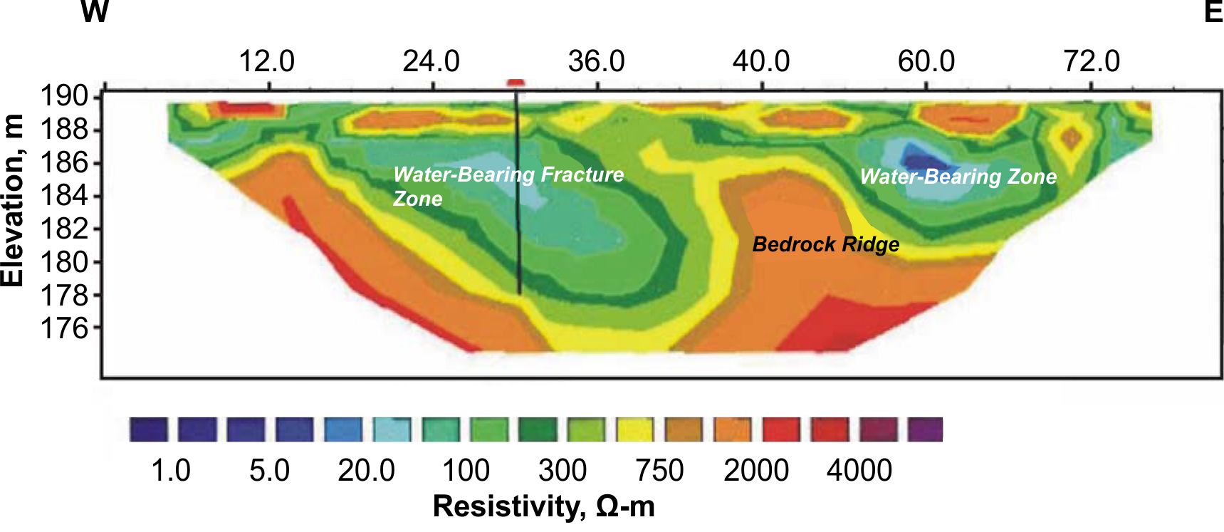
Figure 135. Resistivity data over a fracture zone. (Advanced Geoscience, Inc.)

Advantages: The Automated Resistivity system allows a considerable amount of data to be recorded quite efficiently. Fairly detailed interpretations are possible with this data.

Limitations: Three different methods (traverses, soundings, and automated resistivity system) of using the resistivity method have been discussed above. All of them require electrodes be placed in the ground; thus, the resistivity method is difficult to use in areas where the surface of the ground is hard, such as concrete or asphalt-covered areas. If the ground is dry, water may need to be poured on the electrodes to improve the electrical contact between the electrode and ground.

Clearly the automated resistivity system provides the best interpretation, although it also requires the most effort. With this system, lateral variations in resistivity are recognized and solved for in the inversion process. If data are recorded along a single line, lateral variations in resistivity normal to the line are not accounted for. However, additional parallel lines can be recorded to minimize this potential problem, or a three-dimensional survey can be conducted.

Time Domain Electromagnetic Soundings

Basic Concept: Time Domain Electromagnetic (TDEM) soundings are used to obtain the vertical distribution of resistivity. This method is particularly well suited to mapping conductive layers. To a significant degree, this method has now superseded the resistivity sounding method since it requires less work for a given investigation depth and generally provides more precise depth estimates. However, resistivity soundings are still useful for shallow investigations or when resistive targets are sought.

Data Acquisition: To perform TDEM soundings, a square loop of wire is laid on the ground surface. The side length of this loop is about half of the desired depth of investigation. A receiver coil is placed in the center of the transmitter loop (Figure 120). Electrical current is passed through the transmitter loop and then quickly turned off. This sudden change in the transmitter current causes secondary currents to be generated in the ground. The currents in a conductive layer decay at a slower rate than those in a resistive layer. However, the relationship between the voltage at a particular time after the current is turned off (delay time) and the conductivity and depth of layers under the sounding site is complex, although, longer delay times generally correspond to greater depths.

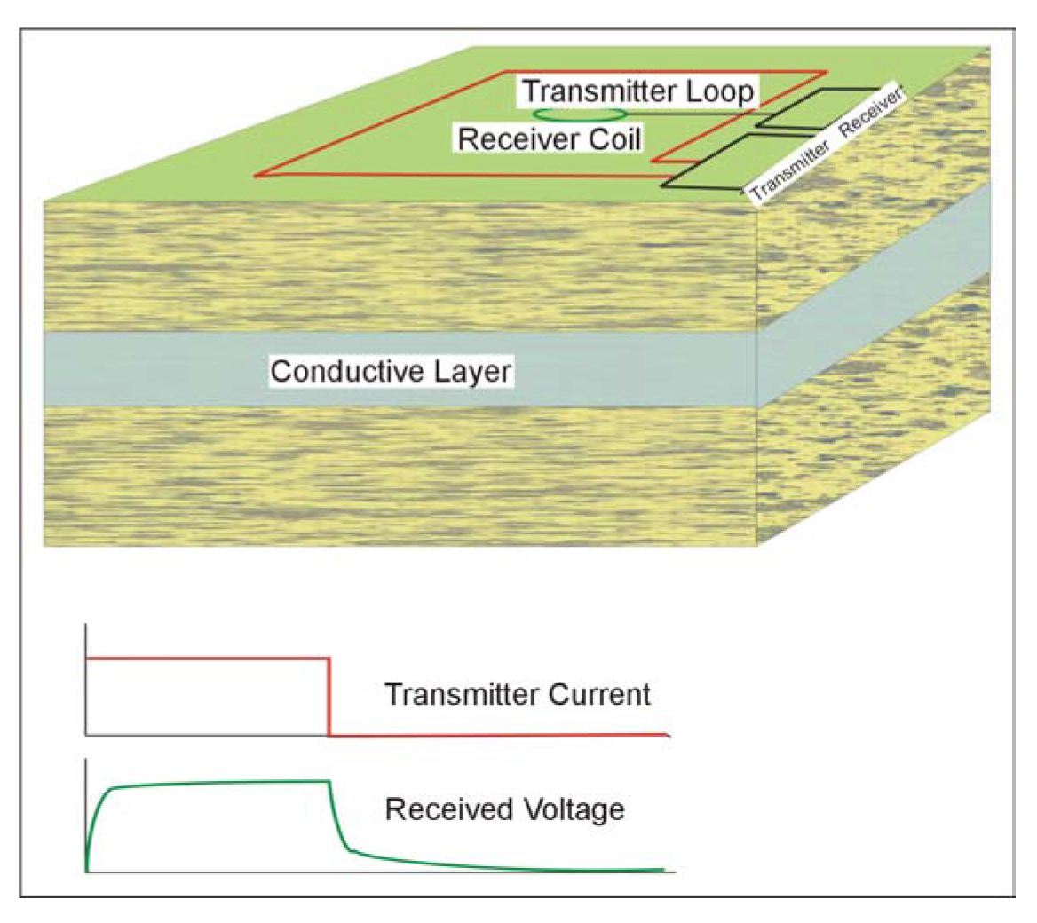
Figure 120. Time Domain Electromagnetic Sounding.

The voltage measured by the receiver coil does not decay instantly to zero when the current is turned off but continues to decay for some time. This decaying voltage is caused by the decaying secondary electrical currents in the ground. The voltage measured by the receiver is then converted to resistivity. A plot is made of the measured resistivity against the time after the transmitter current is turned off (delay time), as illustrated in Figure 121.

The resistivity sounding curve shown in Figure 121 illustrates the curve that would be obtained over three-layered ground. The near-surface layer is fairly resistive. This is followed by a layer having a much lower resistivity (higher conductivity) and causes the measured resistivity values to decrease. The third layer is again resistive.

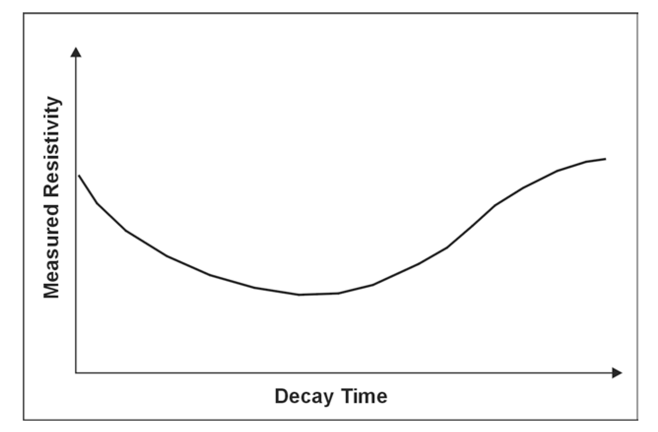
Figure 121. A Time Domain Electromagnetic Sounding curve.

The field layout for TDEM soundings is described earlier. Switched current, as described earlier, is passed through the transmitter loop, and the resulting voltage is measured by the receiver coil. The switching and measuring procedure is repeated many times, allowing the resulting voltages to be stacked, thereby improving the signal-to-noise ratio. This procedure is repeated at different sounding locations until the area of interest has been covered. A sounding curve is plotted for each location showing the measured resistivity against decay time.

Data Processing: Little processing is applied to the data, apart from possibly the removal of bad data points.

Data Interpretation: Interpretation is usually done by inverting the TDEM sounding curves to give interpretations of the resistivity and depths of the layers under the sounding site.

Advantages: The TDEM method is an efficient method for obtaining the subsurface layer resistivities and thicknesses. It should provide an effective method for mapping the groundwater surface providing a resistivity contrast exist with the host materials. It is a more efficient method to use than resistivity soundings when the depths of investigation exceed about 50 meters.

Limitations: The TDEM method is best suited for mapping conductive layers. Groundwater usually increases the conductivity of the rocks and, hence, mapping of conductive layers is needed. If metallic objects (i.e., pipelines), are close to the transmitter loop, electrical currents are induced into these objects by the transmitter loop, and they generate secondary currents and fields. These fields interfere with the electromagnetic fields from the ground and may significantly reduce the interpretability of the data. This method is probably not suitable if the groundwater is less than about 3 meters deep.

At the present time, only one-dimensional interpretation software is available. Therefore, the interpretation assumes that the subsurface layers are horizontal and homogeneous.

Seismic Refraction

Basic Concept: The seismic refraction method can be used to map the water table surface under certain conditions. If the alluvial sediments are fine grained, then the seismic refraction method will probably not be effective because the capillary zone destroys a well-defined seismic velocity contrast between the unsaturated and saturated alluvium. In addition, there may not be a significant velocity contrast between the unsaturated and saturated alluvium. However, if the alluvium is composed of coarse gravel, there will be only a very limited capillary zone. In addition, there will usually be a reasonable velocity contrast between the unsaturated alluvium, which will have a low velocity (500-800 m/s), and the saturated alluvium, which will have a velocity somewhat greater than that of water, which is about 1,400-1600 m/s.

The method requires a seismic energy source, usually a hammer for depths less than 30 meters and black powder seismic guns for depths over 30 meters. The seismic waves then penetrate the overburden and refract along the water table surface. While they are traveling along this surface, they continually refract seismic waves back to the ground surface. These are then detected by geophones placed on the ground surface. Figure 114b shows a seismic recorder instrument, and Figure 114a shows the layout of the instrument, the main seismic waves involved and the resulting time distance graph.

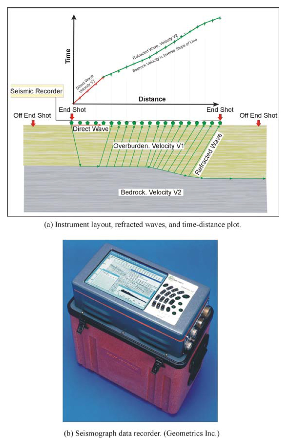
Figure 114. Seismic Refraction: field set up and data recorder.

Data Acquisition: The design of a seismic refraction survey requires a good understanding of the expected depth to the saturated layer. With this knowledge, velocities can be assigned to these features, and a model developed that will show the parameters of the seismic spread best suited for a successful survey. These parameters include the length of the geophone spread, the spacing between the geophones, the expected first break arrival times at each of the geophones, and the best locations for the off-end shots. Knowing the expected first break arrival times is also helpful in the field, where field arrival times that correspond fairly well to expected times help to confirm that the spread layout has been appropriately planned, and that the target layer is being imaged.

Data Processing: The first step in processing/interpreting refraction seismic data is to pick the arrival times of the earliest seismic signal, called first break picking. A plot is then made showing the arrival times against distance between the shot and geophone, called a time-distance graph. An example of such a graph for a two-layered ground (overburden and refractor) is shown in Figure 114a.

The red portion of the time-distance plot in Figure 114a shows the waves arriving at the geophones directly from the shot. These waves arrive before the refracted waves. The green portion of the graph shows the waves that arrive ahead of the direct arrivals. These waves have traveled a sufficient distance along the higher speed refractor (water table) to overtake the direct wave arrivals.

Data Interpretation: Several methods of refraction interpretation are used. In recent years, seismic refraction tomography (SRT) has gained popularity and is now the most common method used for interpreting refraction data. The main benefit with SRT is that it allows for obtaining a picture of the velocity distribution in the subsurface highlighting continuous lateral and vertical changes in velocity rather than assuming a layered model.

The SRT technique involves an automated search for the minimum deviation between the measurements made on the ground and the “virtual” measurements of a synthetic model through an iterative computer process. An example of a SRT velocity model is shown in Figure 114c.

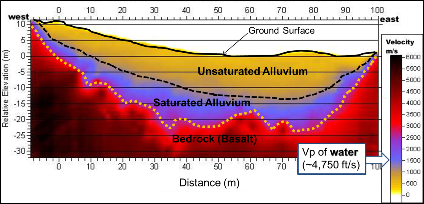
Figure 114c. Bedrock and water table mapping (Image courtesy of USGS).

Another common method of refraction interpretation is called the Generalized Reciprocal Method (GRM) that is described in detail in the Geophysical Methods section. A brief, and simplified, description of the GRM method is presented below. Figure 115 shows the basic rays used for this interpretation.

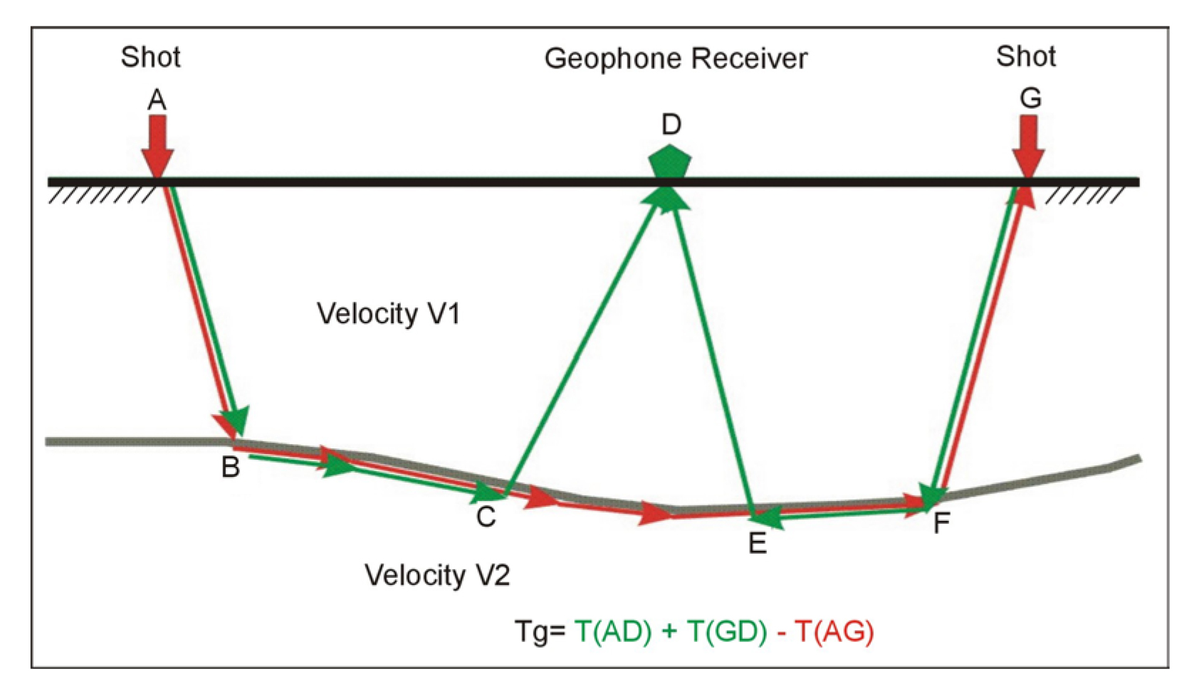
Figure 115. Basic Generalized Reciprocal method interpretation.

The objective is to find the depth to the bedrock under the geophone at D. This is done using the following simple calculations. The travel times from the shots at A and G to the geophone at D are added together (T1). The travel time from the shot at A to the geophone at G is then subtracted from T1. Figure 116 shows the remaining waves after the above calculations have been performed. These are the travel times from C to D added to the travel times from E to D subtracting the travel time from C to E. The sum of these travel times can be shown to be approximately the travel time from the bedrock at H to the geophone at D. Since the velocity of the overburden layer can be found from the time-distance graph, the distance from H to D can be found giving the water table depth.

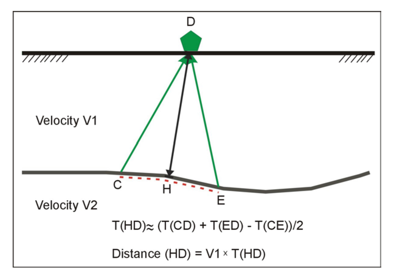
Figure 116. Generalized Reciprocal method interpretation.

Advantages: The seismic refraction method can provide reliable estimates of the water table depths if a velocity contrast exists between the water table and the overlying sediments.

Limitations: It is clearly important that the seismic waves refract from the water table. Usually this will be easily recognized from the field data, assuming the water table provides a refracting surface. However, if refracting layers lie above the water table, these must be recognized if a reliable depth estimate is to be made. If the water table is in the overburden and close to the bedrock, this may obscure the water table arrivals since bedrock has a higher velocity than saturated soils.

Local noise, for example traffic, may obscure the refractions from the bedrock. This can be overcome by using larger impact sources or by repeating the impact at a common shot point several times and stacking the received signals. If noise is still a problem, a larger energy source may be required. In addition, since some of the noise travels as airwaves, covering the geophones with sound absorbing material may also help to dampen the received noise.

Ground Penetrating Radar

Basic Concept: Ground Penetrating Radar (GPR) can be used provided the conditions are appropriate for the method. In order for the method to work, the saturated alluvium must provide a contrast in dielectric properties from those of the unsaturated alluvium. In addition, any clay in the alluvium will significantly attenuate the GPR signal and limit the depth of investigation. Ideal conditions for this method are a dry, sandy overburden. In ideal conditions, the method may penetrate to depths of 15 meters or greater.

The GPR instrument consists of a recorder and a transmitting and receiving antenna. Different antennae provide different frequencies. Lower frequencies provide greater depth penetration but lower resolution. Figure 111 provides a drawing illustrating the GPR system. The transmitter provides the electromagnetic signals that penetrate the ground and are reflected from objects and boundaries, providing a different dielectric constant from that of the alluvium. The reflected waves are detected by the receiver and stored in memory.

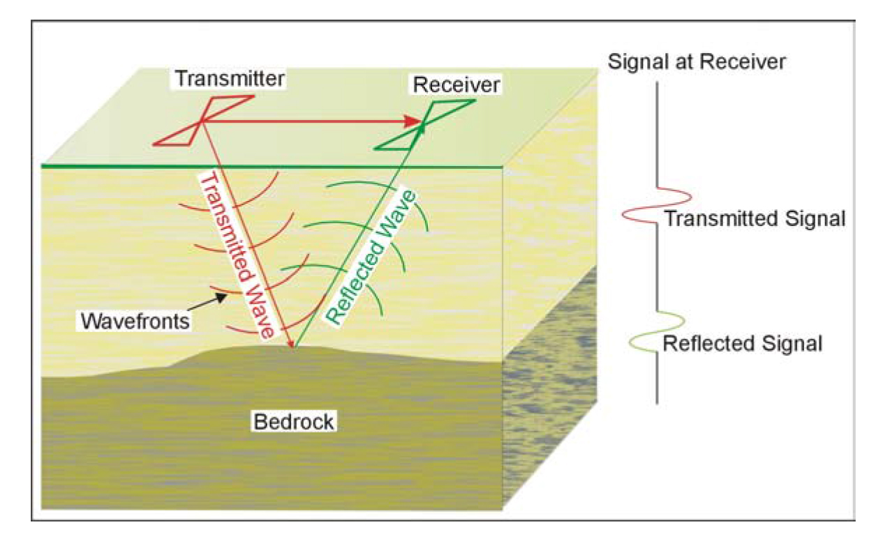
Figure 111. Ground Penetrating Radar System.

Several companies manufacture GPR equipment including Geophysical Survey Systems (GSSI), GeoRadar, Mala GeoScience, and Sensors and Software. Figure 112 shows a typical instrument.

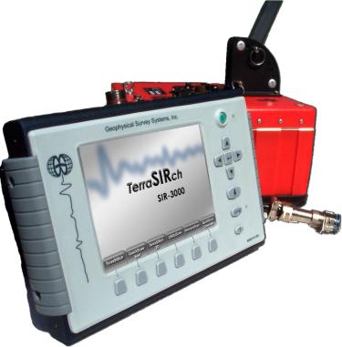
Figure 112. Ground Penetrating Radar instrument. (Geophysical Survey Systems, Inc.)

Any antenna supported by this instrument can be attached and used to collect data. Figure 113 shows a 100 MHz antenna that can be used with the above instrument. The 100 MHz antenna is suited for deeper applications to depths of 15 to 20 m in ideal conditions. This antenna could be used to map the water table depth.

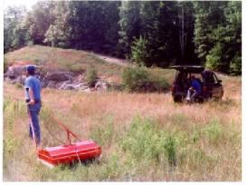
Figure 113. Ground Penetrating Radar. antenna (100 MHz) used in a survey. (MALA GeoScience USA, Inc.)

Data Acquisition: GPR surveys are conducted by pulling the antenna across the ground surface at a normal walking pace. The recorder stores the data as well as presenting a picture of the recorded data on a screen.

Data Processing: It is possible to process the data, much like the processing done on single-channel reflection seismic data. Processes may include distance normalization, horizontal scaling (stacking), vertical and horizontal filtering, velocity corrections, and migration. However, depending on the data quality, this may not be necessary since the field records may be all that is needed to observe the water table.

Data Interpretation: To calculate the depth to the water table, the speed of the GPR signal in the alluvium at the site needs to be obtained. This can be estimated from textbook speeds for typical soil types, or it can be obtained in the field by conducting a small traverse across a buried feature whose depth is known. Once this is known, the depth to the water table can be found from the travel time to the reflector that images the water table and the speed of the GPR signal.

Advantages: GPR data is recorded simply by pulling the system across the area of interest. Data can be viewed in the field allowing recording parameters, such as antenna frequency, changes to be made if needed.

Limitations: Probably the most limiting factor for GPR surveys is that their success is very site specific and depends on having a contrast in the dielectric properties of the target compared to the host overburden, along with sufficient depth penetration to reach the target. However, it is likely that in many cases the water table will provide a dielectric contrast with the unsaturated overburden, and depth of penetration is probably the most important factor. Clay in the overburden will usually severely limit the depth penetration of the GPR signals.

Nuclear Magnetic Resonance

Basic Concept: The Nuclear Magnetic Resonance (NMR) method is also known as the Proton Magnetic Resonance (PMR) method. On this website, the term NMR will be used. This method is still being developed, although commercial equipment for taking NMR measurements is currently available. The NMR method is based on the excitation of protons in the subsurface water in the presence of the Earth's magnetic field.

The instrument consists of a transmitter and receiver. The transmitter drives alternating current at the proton resonance frequency through a loop of wire laid on the ground. The current is abruptly terminated, and the NMR signal is then measured using the transmitter wire loop as a receiving antenna. This procedure is repeated several tens to a few hundreds of times, during which the NMR signal is recorded and averaged to improve the signal-to-noise ratio. The signal is interpreted in terms of hydrological parameters as a function of depth. Figure 164 shows the basic physics of the NMR (or PMR) method.

S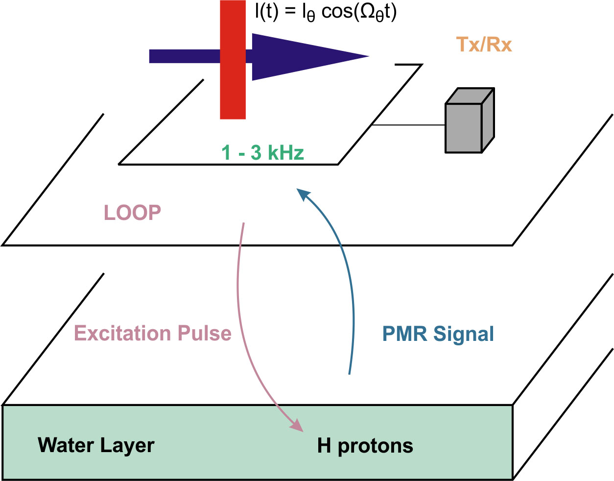

Figure 164. Schematic of the Nuclear Magnetic Resonance method. (IRIS Instruments)

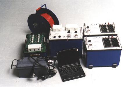
Figure 165. Instrument for measuring Nuclear Magnetic Resonance. (IRIS Instruments)

The transmitter/receiver loop provides the electromagnetic pulses that excite the protons in groundwater. These protons then decay during the transmitter current off time, and the field from this decay is detected by the same loop of wire now acting as a receiver. The data are stored in the control transmitter/receiver (Tx/Rx) box. Figure 165 shows the instruments for measuring NMR.

Data Acquisition: NMR surveys are conducted by laying a loop of wire on the ground. The size of the loop depends on the Pulse Moment (current multiplied by time while current is transmitted) during the measurement, which determines the depth of investigation. A typical loop size for investigation depths to 100 m might be 100 m side length. Rectangular pulses of alternating current are passed through the wire with a frequency equal to that of the proton resonance in the Earth's magnetic field, as illustrated in Figure 165. Signals are received by the wire loop while the current is off.

Six basic steps define the general procedure for carrying out NMR soundings.

1. Measure the strength of the Earth's magnetic field. From this, the frequency of the signal to transmit can be found.
2. Transmit a pulse of current using the wire loop at the frequency found in step 1.
3. Measure the amplitude of the water NMR signal.
4. Measure the time constant of the signal
5. Change the pulse intensity to modify the depth of investigation.
6. Interpret the data using an inversion program.

Data Interpretation: An example of the field data and interpretation is shown in Figure 166. The Figure shows the field data from a sounding, along with the interpretation. The field data curve (left plot) shows the noise level (blue circles), the measured field data (black squares) and the interpretation fit (red line).

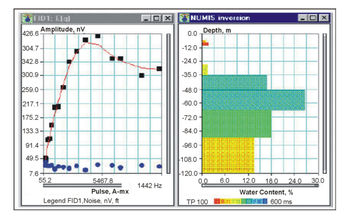
Figure 166. Field data and interpretation of a Nuclear Magnetic Resonance survey. (IRIS Instruments)

There are four important items concerning the interpretation of the results.

1. The method detects water. No signal is observed if no water is present.
2. The amplitude of the NMR signal is related to the variation in water content with depth.
3. The decay time constant of the NMR signal is related to the variation in mean pore size against depth.
4. The phase shift between the NMR signal and the current is related to the layer resistivity variation with depth.

The right-hand graph shows the interpretation, presenting a plot of porosity versus depth. Since water within the rock pores is required for the method to work, this plot shows the water content of the rock layers.

Advantages: The main advantage of the NMR method is that it responds only to the protons within water.

Limitations: The method requires large currents to be used when transmitting, necessitating large-diameter wire. Therefore, the wire is heavy and can be difficult to lay out in any area with bush or significant topography. Probably the biggest limitation is the influence of electrical noise, such as power line noise. Generally, soundings need to be at least 1,000 m from any power line. If magnetic minerals are present in the subsurface, these destroy the uniform magnetic field required to initialize the proton oscillations in the groundwater. When these magnetic minerals are present, the NMR method is ineffective.

Methods: Groundwater Flow

Self Potential

Basic Concept: The only geophysical method used to detect groundwater flow is the Self Potential (SP) method. This method measures naturally occurring electrical potentials on the ground surface, some of which may result from the flow of groundwater in porous medium.

Self-Potential voltages have a number of causes. The largest potential probably results from mineralization where negative SP anomalies of hundreds of millivolts can occur. Natural electrical potentials can also occur due to telluric currents. These are large currents flowing in the earth that result from electrical activity in the earth's atmosphere and beyond.

Figures 167 and 168 show the SP potentials over a fracture zone when water is flowing into and out of the fracture zone. When water flows into a fracture (Figure 168) a negative SP anomaly is observed above the flowing water. Conversely, when water flows out of the fracture zone (Figure 168), there is a positive SP anomaly.

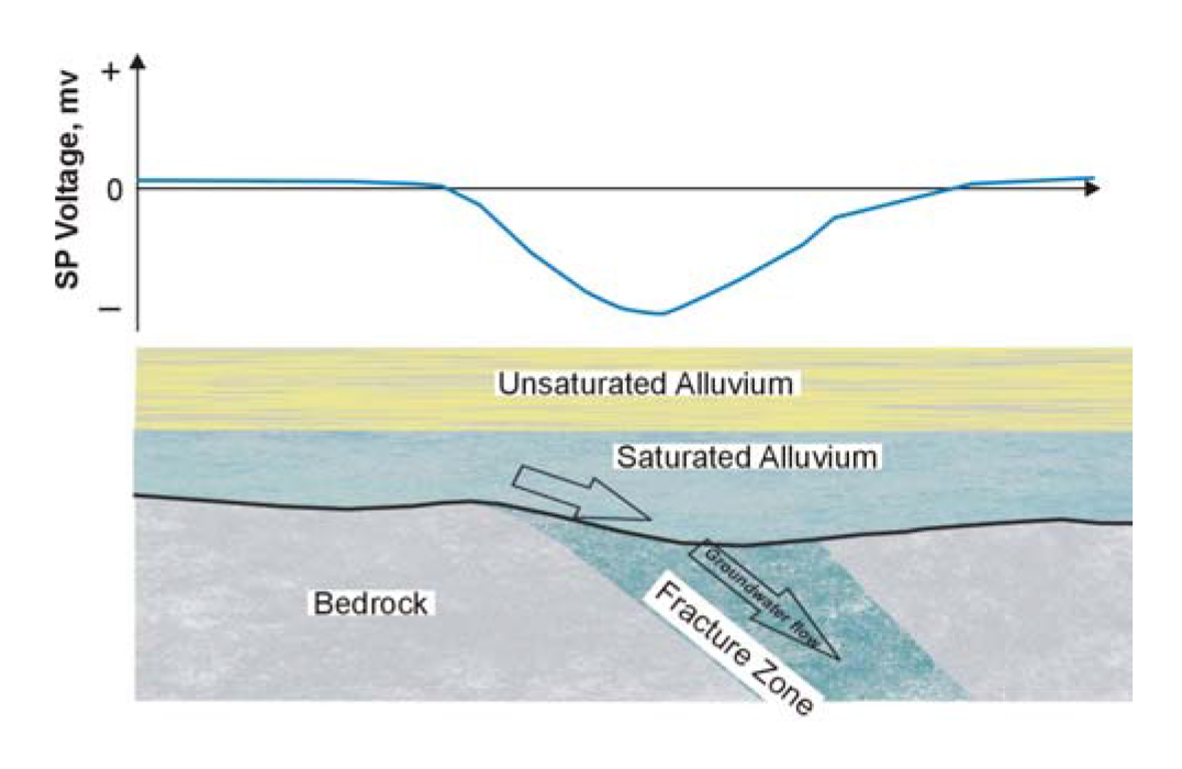
Figure 167. Self-Potential anomaly expected over water flowing into fracture zone.

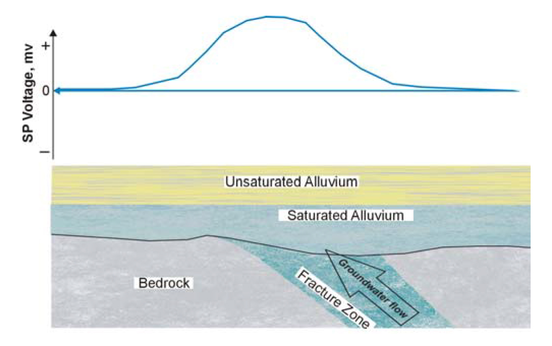
Figure 168. Self-Potential anomaly expected over water flowing out of a fracture zone.

Data Acquisition: There are two techniques for recording SP data. These are illustrated in Figure 169. One requires an electrode (normally a porous pot or stainless steel spike) at a permanent reference point, called the reference electrode in Figure 169. Long wires are required to connect a second electrode (roaming electrode) to the reference electrode. The roaming electrode is then moved along the desired traverse while taking voltage readings between the two electrodes. This system is called the remote electrode system in Figure 169. This provides the SP voltage at each station with reference to the reference electrode. The second technique is much easier to use in the field. There is a fixed distance between the two electrodes, and the electrode system is moved in increments along the traverse. This system is called the dipole system in Figure 169.

Data Processing: The measured voltages usually require little processing.

Data Processing: Interpretation is usually done from profiles of the measured voltage against distance, searching for the anomalies shown in Figures 167 and 168. Some modeling is also available for a more quantitative interpretation.

Advantages: The SP method is very simple to perform in the field and uses inexpensive equipment.

Limitations: SP anomalies can result from several other factors, some of which give larger anomalies than those due to water flow. However, the method is simple and easy to apply. The method will not work near grounded structures or near grounded metal features such as fences since these may generate potentials due to corrosion. In addition, surveys near electrical groundings will likely be ineffective.

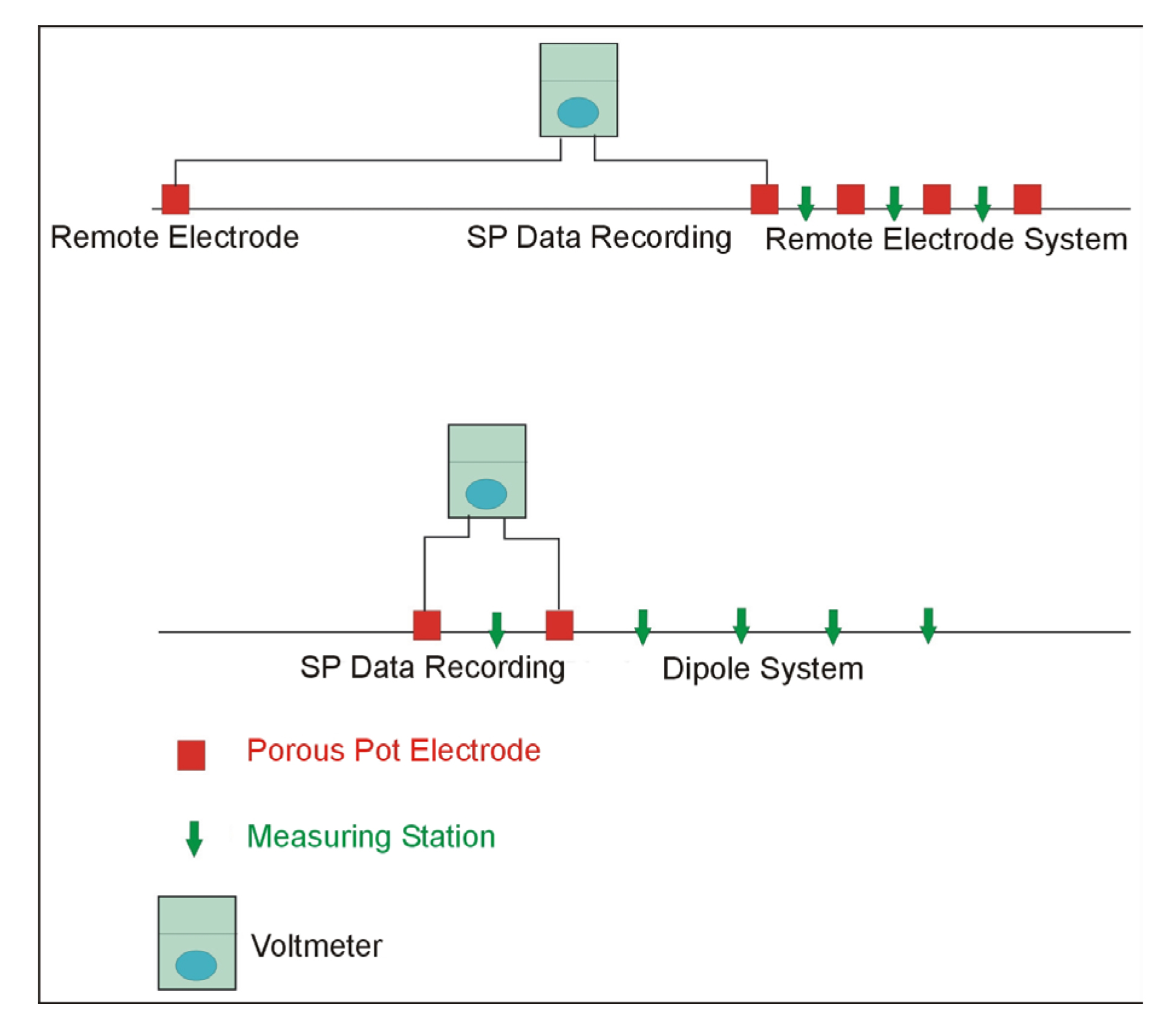
Figure 169. Methods of recording Self Potential data.

Electroseismic

Basic Concept: The Electroseismic method (also called the Seismoelectrical method) is based on the generation of electromagnetic fields in soils and rocks by seismic waves. Although the method is not reported to detect groundwater flow, it is reported to measure permeability and, therefore, to detect the potential for groundwater flow.

As the seismic (P or compressional) waves stress earth materials, four geophysical phenomena occur:

1. The resistivity of the earth materials is modulated by the seismic wave.
2. Electrokinetic effects analogous to streaming potentials are created by the seismic wave.
3. Piezoelectric effects are created by the seismic wave.
4. High-frequency audio and high-frequency radio frequency impulsive responses are generated in sulfide minerals (sometimes referred to as RPE).

The dominant application of the Electroseismic method is to measure the Electrokinetic effect or streaming potential (item 2, above). Electrokinetic effects are initiated by sound waves (typically P-waves) passing through a porous rock inducing relative motion of the rock matrix and fluid. Motion of the ionic fluid through the capillaries in the rock occurs with cations (or less commonly, anions) preferentially adhering to the capillary walls, so that applied pressure and resulting fluid flow relative to the rock matrix produces an electric dipole. In a non-homogeneous formation, the seismic wave generates an oscillating flow of fluid and a corresponding oscillating electrical and EM field. The resulting EM wave can be detected by electrode pairs placed on the ground surface.

Surface seismic sources and measurement electrode pairs are generally used to measure the Electrokinetic effect. Borehole systems also have recently been developed. A hammer blow or small explosive (black powder) are typically used for the seismic source. Two short (few meters) electrode pairs are typically located collinear and symmetric to the seismic source. Stacking of repeat seismic "shots" is often used to improve signal to noise.

Only one company was found that produces a commercially available Electroseismic prospecting system, GroundFlow Ltd. in the UK. This system has been used mainly for field demonstration purposes and research and development studies. Very few detailed case histories are available to web manual the performance of the system. The Electroseismic system made by GroundFlow is called "GroundFlow 1500." The main equipment components are a combined computer-receiver, antenna cables and electrodes, and the trigger cable. The Groundflow 1500 instrument is shown in Figure 170.

Figure 170. The GroundFlow 1500 Electroseismic system instrument. (Groundflow, Ltd.)

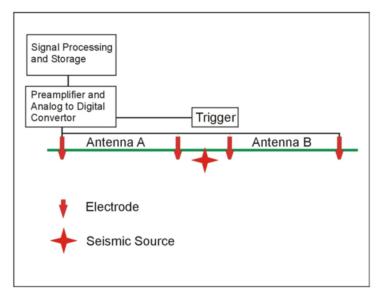
Figure 171. System layout for Electroseismic surveys.

The computer-receiver contains a preamplifier, analog to digital converter and power supply system to measure the voltages induced in the grounded dipoles. The system layout used by GroundFlow is shown in Figure 171.

The hammer and plate seismic source is used along with two pairs of electrodes arranged in a straight line with electrodes offset (from the center of the array) by 0.25 and 2.25 m. The seismic source is positioned in the center of the array. Larger electrode spacings can be used; however, they are typically centered in pairs around the shot point and are generally less than about 10 m in length. Timing of the measurement is achieved by a hammer trigger. The signal is acquired with the instrument shown in Figure 7. Measurements are made for a period of 400 ms after triggering. The last 200 ms of the record is used as a sample of background noise and is subtracted from the first 200 ms of signal to remove the first, third, and fifth harmonics of the background noise at the receivers. This noise is typically from power lines.

Data Acquistion: Measurements are recorded using the instrument and system setup described above. Data processing consists of stacking repetitive hammer (or explosive) shots and removing power line and other noise. This processing is conducted on the computer-receiver while in the field. Depending upon field conditions, up to 20 soundings can be conducted in a day. It is expected that measurement time will increase proportionally with stacking times, and that long stacking times would be needed in the vicinity of power lines.

Data Processing: The signal files are processed to give a sounding plot of permeability and porosity against one-way seismic travel time. Values for a simple seismic velocity model are required to allow time to depth conversion. The resulting logs against depth are displayed in the field.

Output from the Electroseismic inversion is typically a plot showing hydraulic conductivity versus depth. This interpretation assumes a one-dimensional layered earth. In theory, the inversion also can derive fluid conductivity and fluid viscosity from the rise time of the signal. Where many soundings are measured in close vicinity, a pseudo-2-D cross section can be generated.

The maximum depth of penetration of Electroseismic measurements is stated to be about 500 m depending upon ambient noise and water content. Lateral resolution is not stated in the literature but is expected to be on the order of the depth of exploration. No information was found regarding the vertical resolution of the method.

Advantages: Since this method is primarily used by only one contractor, and little independent data is available about the results, it is not known what the advantages of the method are.

Limitations: The Electroseismic method is apparently susceptible to electrical noise from nearby power lines. Typical Electroseismic signals are at the microvolt level. The Electroseismic signal is proportional to the pressure of the seismic wave. Thus, it would seem possible to increase the signal by using stronger seismic sources. This is not mentioned in the literature. Although Electroseismic soundings are reported to have a maximum exploration depth of about 500 m, no examples have been shown with results from deeper than about 150 m.

Borehole HydroPhysical™ Logging

HydroPhysical™ logging is a technology used for evaluating the vertical distribution of permeability and water quality in wells. Using this procedure, interval-specific contaminant concentrations, hydraulic conductivity, and flow rates are assessed with great accuracy and sensitivity. Cross-hole flow evaluations are also possible with this method.

Basic Concept: Borehole fluids are replaced or diluted with deionized (DI) water. During this process, profiles of the changes in fluid electrical conductivity (FEC) of the fluid column are repeatedly recorded using a highly sensitive FEC/temperature logging probe. These changes occur when electrically contrasting formation water is drawn back into the borehole by pumping or by native formation pressures (Figure 172). A downhole wireline simultaneously measures FEC and temperature of the emplaced fluid.

Data Acquisition: Truck mounted pumping, logging, and deionization equipment is rigged up on the screened or open borehole. FEC logs are recorded before, during, and after emplacement of deionized water. Formation water recovery may be monitored during native (ambient) or pumping (stressed) conditions. Natural borehole fluid is extracted and stored, as the DI water is injected.

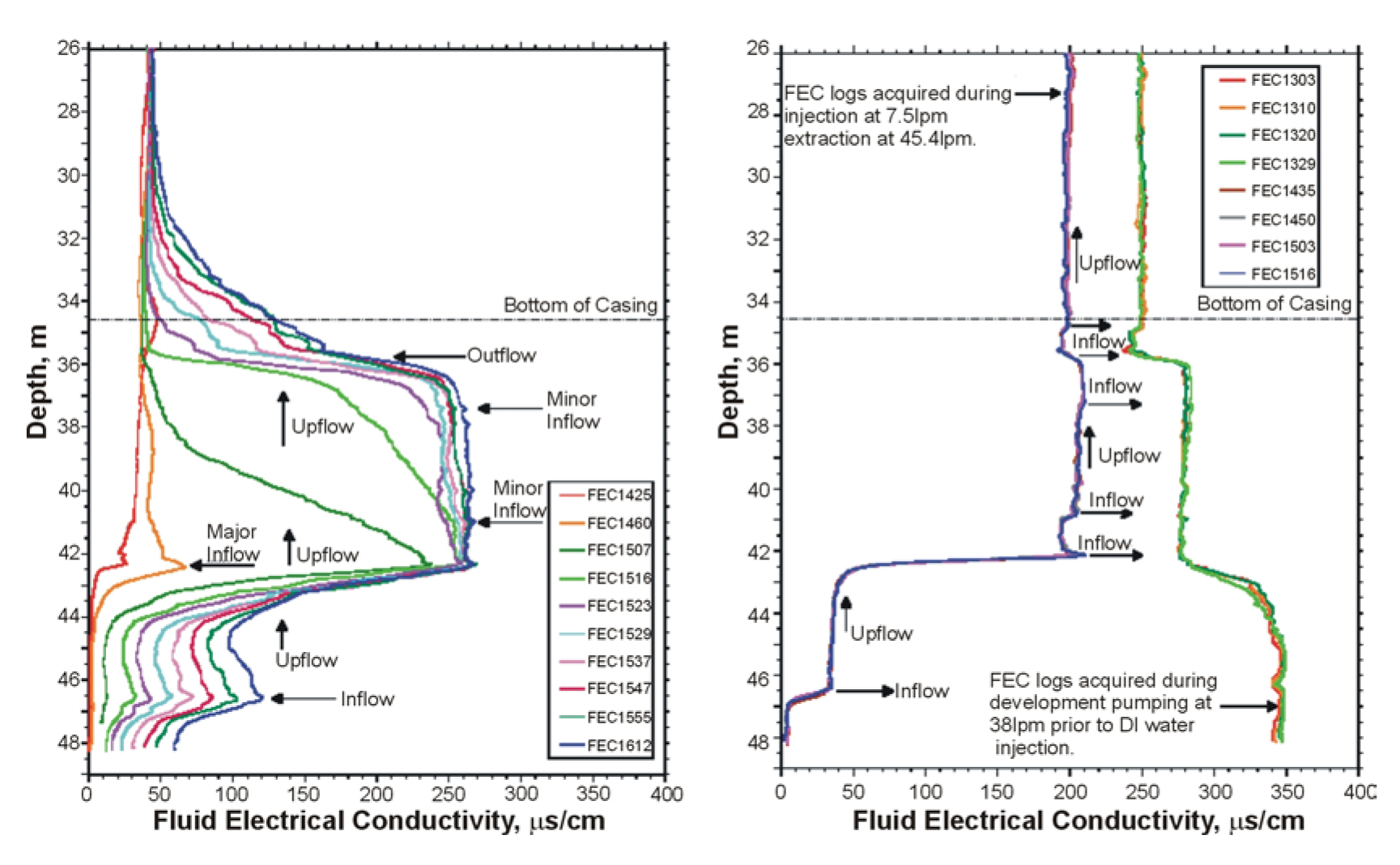
Figure 172. Examples of ambient flow Characterization and 10 gpm production test, respectively. (Layne Christensen, Colog)

Data Processing and Interpretation: Software developed in conjunction with Lawrence Berkley laboratory is used to perform modeling showing upflow, downflow, ambient horizontal flow, outflow and inflow quantities of formation fluid for specific intervals. Using the mass-balance equation, and numerical modeling of FEC logs, interval-specific flow rates and the hydrochemistry of the water-bearing intervals can be determined.

Advantages: HydroPhysical™ logging provides a wide range of interval-specific flow rates that can be quantified from 0.01 to 2,000+ gpm. The technology is more cost effective than packer testing, and it is applicable in low and high yield bedrock, alluvial settings, karst, and volcanic acquifers. HydroPhysical™ logging allows the identification and evaluation of ambient horizontal and vertical flows, and ambient horizontal velocities can be converted into Darcian velocities for the aquifer.

Limitations: Concerns about fluid discharge are continuing to mount as environmental responsibility moves to the forefront. Fluid extracted during DI emplacement must be disposed of. Disposal may require permission for ground or stream discharge from the local water authority, or it can require storage, and removal for processing, if the presence of contaminants is possible.