Fractures in bedrock occur most often in competent rocks that are not able to adjust to the stresses placed upon them. Shales and clays are less likely to be fractured than harder rocks such as limestone and metamorphic rocks. Limestone may also develop solution cavities and fissures in addition to fractures. Since geophysical methods will rarely be able to detect individual fractures unless they are very large, regions of fracturing, called fracture zones, are more likely to provide geophysical targets. Weak zones are regions or zones where the bedrock cannot tolerate significant compressive stress without deformation. They often have physical properties similar to those of fracture zones but may be more extensive. Weak zones may occur if the bedrock surface is a series of dipping layers with some layers being less competent than other layers. This may occur if one of the dipping layers is more prone to weathering than its host layers. Metamorphic rocks may exhibit weak zones due to differential weathering. In addition, shale or clay layers under a thin layer of more competent rocks may constitute a weak zone, as illustrated in Figure 134a. In this case, stresses placed on the thin limestone layer may require more support from the deeper shale/clay layer than it can provide. Another example of a potential weak zone is presented in Figure 134b.

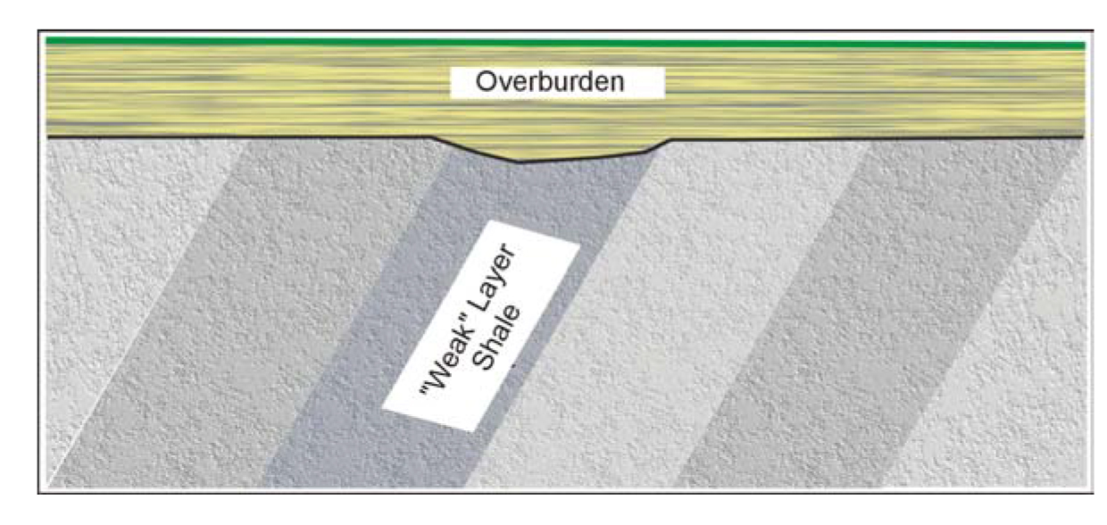
(a) Bedrock surface formed from a series of dipping layers.

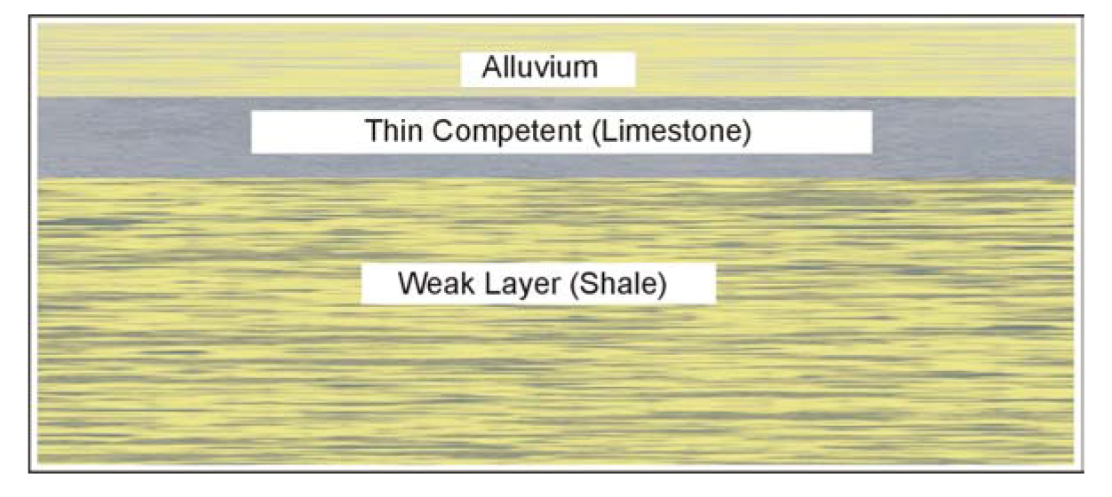
(b) Weak zone comprising a thin, competent limestone layer overlying a weak shale layer.

Figure 134. Two conceptual examples showing weak zones.

Geophysical methods are commonly used to find fractures in bedrock and can also be used to find weak zones. Generally, fracture zones are likely to contain more moisture than non-fractured bedrock, making them more electrically conductive, as well as having a lower seismic velocity. Fracture zones may provide the following physical parameter differences compared to the host rock:

1. Lower resistivity (higher conductivity).
2. Lower seismic velocity.
3. Bedrock topographic depressions due to fracturing and weathering.

In addition, the fracturing may cause scattering of seismic and Ground Penetrating Radar (GPR) waves. It is also possible that these areas will have lower densities that could theoretically produce gravity anomalies. However, many other interpretations of a gravity anomaly are possible and, because of this and the time-consuming nature of gravity surveys, these are not discussed further.

These parameters also generally apply to weak zones apart from the limestone/shale layering described above. In this case, the limestone will have a high resistivity and seismic velocity and the shale a low resistivity and seismic velocity. Mapping these layers requires the vertical distribution of resistivity, or velocity, rather than the horizontal distribution of these parameters as in the search for fracture zones. The methods used for detecting the limestone/shale layers will be described in the appropriate section below.

The physical parameters of weak zones that are useful for geophysical surveys are similar to those for locating fractures. In the case shown in Figure 134a, these include a higher conductivity and a bedrock depression. However, depending on the complexity and thickness of the dipping layers, this weak zone may be more difficult to detect than fractures in horizontally layered bedrock. This is because the layering in the host bedrock may cause more varied physical parameters than those where the bedrock is horizontal and uniform. These variations may cause geophysical "noise" making it more difficult to observe the attributes of the weak zone.

There are many different geological conditions in which fractures and weak zones occur. The two weak zone cases and the fracture zone case are simple examples used to illustrate the application of geophysical methods. However, because of the complexity of geological conditions, for field surveys each case needs to be evaluated individually, and the appropriate geophysical method selected, since many factors influence the choice of geophysical method, or methods, to use.

The geophysical methods generally appropriate for locating fracture zones and weak zones are listed below.

1. Resistivity measurements (soundings and traverses).
2. Time Domain Electromagnetic Soundings.
3. Conductivity measurements.
4. Common offset surface (Rayleigh) waves.
5. Shear wave reflection surveys.
6. Seismic refraction surveys.
7. Ground Penetrating Radar surveys.
8. Very Low Frequency Electromagnetic surveys (VLF).

In the above list, resistivity and conductivity measurements are separated because they involve different instruments, and there are important differences in the application of the techniques.

Methods

Since all of these techniques, except VLF surveys, have been discussed in detail earlier in this section, only the important factors for locating fractures and weak zones will be discussed in this section.

Resistivity

Basic Concept: The resistivity method can be used to locate fracture zones and weak zones if they have a resistivity contrast with the host rocks. There are two common resistivity methods: soundings and traverses. Resistivity traverses are used to map changes in the bedrock and overburden resistivity. If the overburden resistivity does not change laterally, the method can be used to map variations in the elevation of the bedrock surface. Resistivity traverses are often done using only one electrode spacing and, therefore, do not provide the variation of resistivity with depth. Resistivity soundings provide the resistivities and depths of the layers under the sounding site. Lateral variations in resistivity, or conductivity, can be obtained much more efficiently using electromagnetic methods with instruments such as the EM31 and EM34. Hence, resistivity traverses using one electrode spacing are rarely used and will not be discussed further. However, automated resistivity systems are now available that record data from several different electrode spacings very efficiently, combining both traverse and sounding data.

These newer instruments, called automated resistivity systems, use electrodes that are addressable by a central control unit. This means that a large number of electrodes can be placed in the ground prior to starting the survey and connected to the central control unit. The data recording parameters and the electrode array to use are input to the central control unit. Once the electrodes are all connected, the measurements are automatically recorded by the central control unit. Resistivity soundings provide useful information and will be discussed in this section. Resistivity traverses have now largely been replaced by conductivity measurements, since these are much easier to acquire.

The resistivity of the ground is measured using a number of electrode arrangements, some of which are illustrated in Figure 90. In all of these arrays, current is injected into the ground using two electrodes and the resulting voltage is measured using the remaining two electrodes.

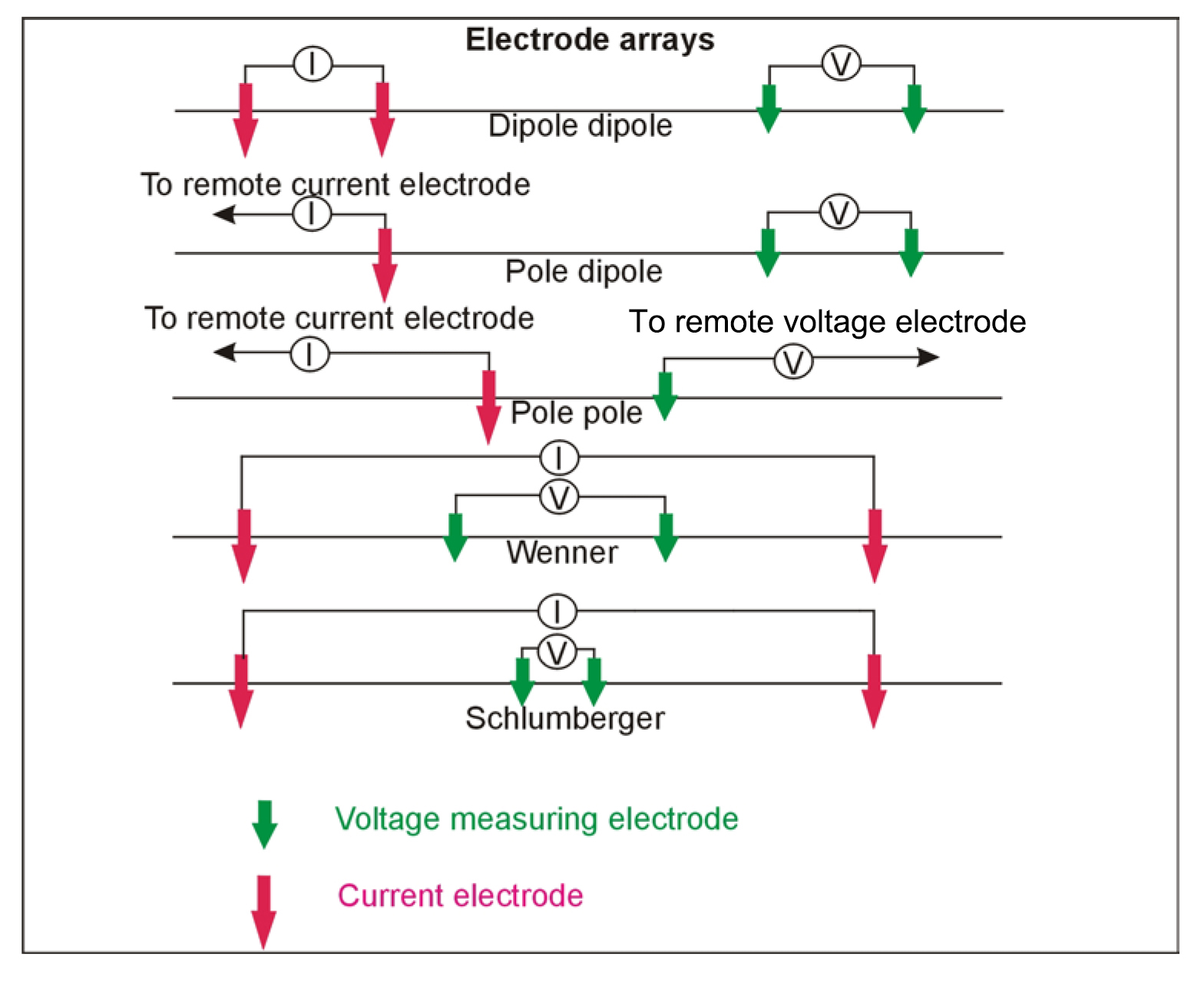
Figure 90. Electrode arrays used to measure resistivity.

The electrode arrays are used for different types of resistivity surveys. The Schlumberger array is often used for resistivity soundings, as is the Wenner array. The Pole-pole array provides the best signal, but is cumbersome because of the long wires required for the remote electrodes and is rarely used. The Dipole-dipole array was originally used mostly by the mining industry for induced polarization surveys. Readings were taken using several different separations of the voltage and current dipoles providing measurements of the variation of resistivity with depth. Long lines of data were recorded requiring many readings. This array has now become common for resistivity surveys using the automated resistivity systems. If more signal (voltage) is needed than can be provided with the Dipole-dipole array, the Pole-dipole array can be used.

Resistivity Soundings

Figure 91 shows one of these electrode arrangements, called the Schlumberger array, and illustrates its use for obtaining a resistivity sounding.

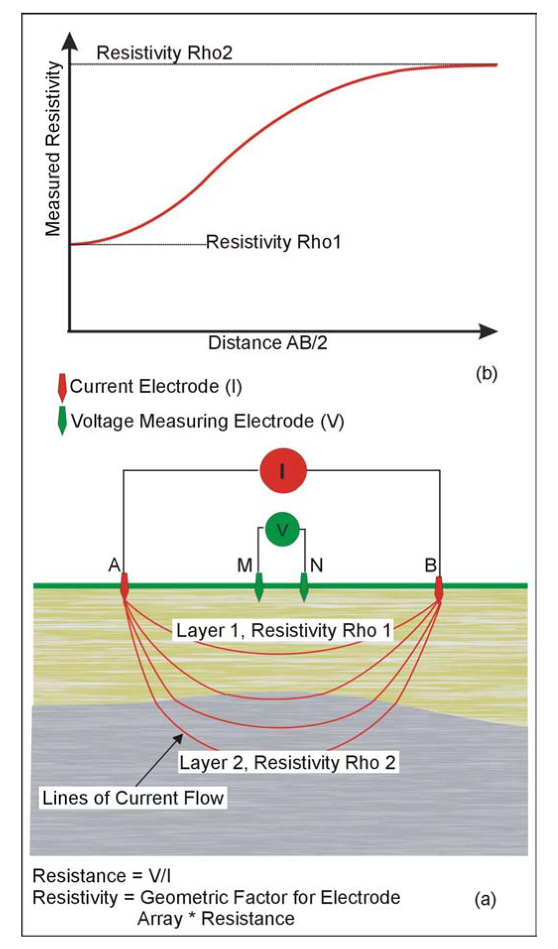
Figure 91. Electrode array for (a) measuring the resisivity of the ground, and (b) a resisitivity sounding curve.

Data Acquisition: In Figure 91a, current is passed into the ground using the two electrodes labeled A and B. The voltage that results from this current is then measured using electrodes M and N. Using the amount of current passed into the ground along with the voltage and a geometric factor for the electrode layout, the resistivity of the ground is calculated. The electrode array is then expanded, making the current penetrate deeper into the ground, and another reading is taken. This procedure is repeated for many electrode spacings providing a set of resistivity values for each of these spacings. These values are plotted on a graph of resistivity against electrode spacing, as illustrated in Figure 91b. This graph shows that, at small electrode spacings, the measured resistivity approaches that of the overburden, whereas at large electrode spacings, the measured resistivity approaches that of the bedrock. The resistivity curve is interpreted using software that provides a resistivity model (depths and resistivities) whose resistivity calculations match the field data.

Resistivity soundings are used to measure the vertical distribution of resistivity in the ground, and hence can be used to map the existence of a conductive shale layer that may occur beneath a more competent layer. Resistivity soundings alone are probably not a useful method for locating fractures. When conducting the survey, it is advisable to plot the measured resistivity versus electrode spacing in the field to ascertain that the deeper layers of interest have been observed.

Data Processing: Usually little processing is needed although bad data points may be removed.

Data Interpretation: Resistivity data are interpreted using software that calculates the sounding curve from a resistivity model. The interpreter inputs a preliminary model, and the computer calculates the sounding curve from this model and evaluates the fit of this model data to the field data. It then changes the model to provide an improved fit and recalculates the resistivity curve. The process, called inversion, is repeated until the curve from the model matches that from the field data.

Advantages: Resistivity soundings are probably more useful than seismic refraction method for locating weak zones, since weak zones are likely to have a lower velocity than the overlaying rocks and seismic refraction will not see the top of the lower velocity layer.

Limitations: Since electrodes have to be planted in the ground, this can be a problem is dry or rocky areas. In such conditions, water may need to be poured onto the electrodes in order to lower the resistance between the electrode and the ground.

Automated Resistivity Systems

Data Acquisition: As mentioned previously, newer resistivity systems are now available that make taking resistivity measurements much more efficient, and by taking many measurements at different electrode spacings along a traverse, these systems are able to build a comprehensive picture of the subsurface, combining both lateral and vertical variations in resistivity. Figure 201 shows the Sting/Swift automated resistivity measuring system. To take resistivity measurements, the electrodes along a traverse are inserted into the ground and connected to the wires leading the controller. The controller is programmed with the desired electrode array to use along with other factors and then instructed to take the measurements.

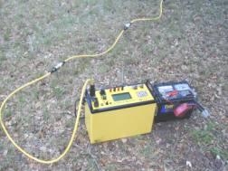
Figure 201. String-Swift Resistivity Measuring System. (Advanced Geosciences, Inc.)

Data Processing: Usually little processing is applied to the data, apart from removing any bad data points.

Data Interpretation: Data from these systems are interpreted by using software that calculates the theoretical resistivity data from a resistivity/depth model, thus enabling a model to be developed that produces data that matches the field data, a process called inversion. However, much information can be gained visually. An example of the results from such a survey is presented in Figure 135. These data show two low-resistivity zones, one of which was shown to be a water- filled fracture zone. The data have been inverted showing the resistivity variation, both laterally and vertically, against depth.

Fracture zones can also be located using a method called Azimuthal Resistivity surveys. In this method, resistivity is measured using an appropriate electrode array and spacing, say the Schlumberger array. The array is then rotated about its center a few degrees, and another reading taken. This process is repeated until readings have been taken as the array rotates through 360 degrees. Variations in resistivity as the array rotates are used to locate fracture zones. However, the method assumes that the bedrock surface is fairly flat, and that there are no resistivity changes in the overburden. Many azimuthal soundings will be required to adequately cover an area. Data recorded with the automated resistivity system probably provides data that offer a better interpretation, and the system is probably more efficient.

Advantages: Using the Automated Resistivity systems, fairly comprehensive data sets can be efficiently recorded and interpreted. Provided the geology is appropriate these systems can be used to locate fractures and weak zones.

Limitations: Three different methods (traverses, soundings, and automated resistivity systems) of using the resistivity method have been discussed above. All of them require electrodes be placed in the ground; thus, the method is difficult to use in areas where the surface of the ground is hard, such as concrete or asphalt-covered areas. In addition, if the ground is dry, water may need to be poured onto the electrodes to improve the electrical contact between the electrode and the ground.

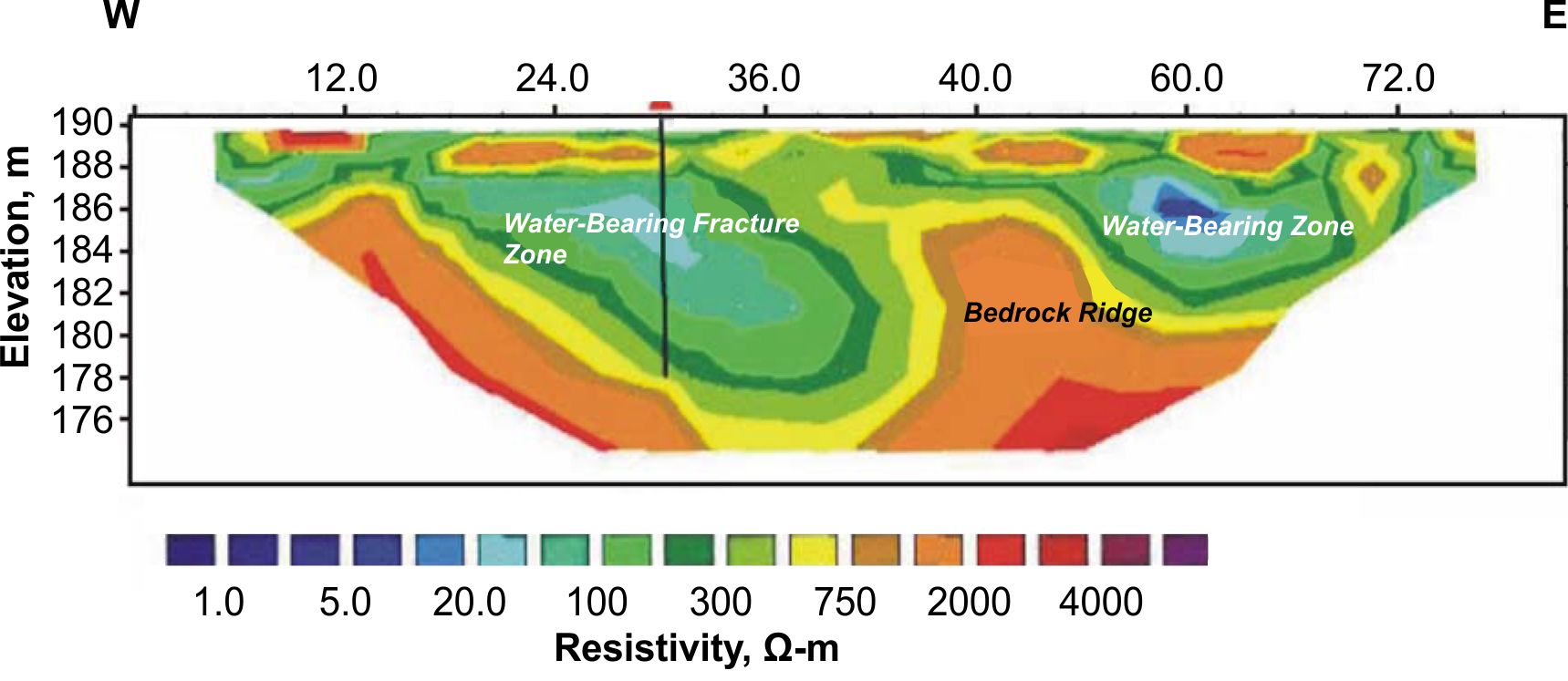
Figure 135. Resistivity data over a fracture zone. (Advanced Geoscience, Inc.)

Resistivity soundings are a useful tool and can provide the resistivities and depths of layers under the sounding site. However, the interpretation assumes horizontal layers with no lateral variations in resistivity. If this is not the case, the interpretation will be incorrect. Generally, with the Schlumberger array, the separation between the current electrodes will need to reach a maximum of about three times the investigation depth. If the bedrock is 15 m deep, the current electrodes will need to be spaced up to 45 m apart.

Clearly, the automated resistivity system provides the best interpretation, although it also requires the most effort. With this system, lateral variations in resistivity are recognized and resolved in the inversion process. Since the data are recorded along a line, the interpretation necessarily assumes that there are no variations in ground resistivity normal to the line, which is probably not true. Thus, errors in the interpretation can occur, depending on the resistivity variations normal to the survey line. This problem can be minimized by conducting parallel traverses or by conducting three-dimensional surveys.

Time Domain Electromagnetic Soundings

Basic Concept: Time Domain Electromagnetic soundings (TDEM) are used to obtain the vertical distribution of resistivity. This method is particularly well suited to mapping conductive layers. To a significant degree, this method has now superseded the resistivity sounding method since it requires less work for a given investigation depth and generally provides more precise depth estimates. However, resistivity soundings are still useful for shallow investigations or when resistive targets are sought.

TDEM soundings are an electromagnetic method used to provide the vertical distribution of resistivity within the ground. A square loop of wire is laid on the ground surface. The side length of this loop is about half of the desired depth of investigation. A receiver coil is placed in the center of the transmitter loop. Electrical current is passed through the transmitter loop and then quickly turned off. This sudden change in the transmitter current causes secondary currents to be generated in the ground. These decaying currents have associated decaying electromagnetic fields that produce a voltage in the receiver coil on the ground surface. The TDEM field layout, transmitter current, and received voltage are illustrated in Figure 120.

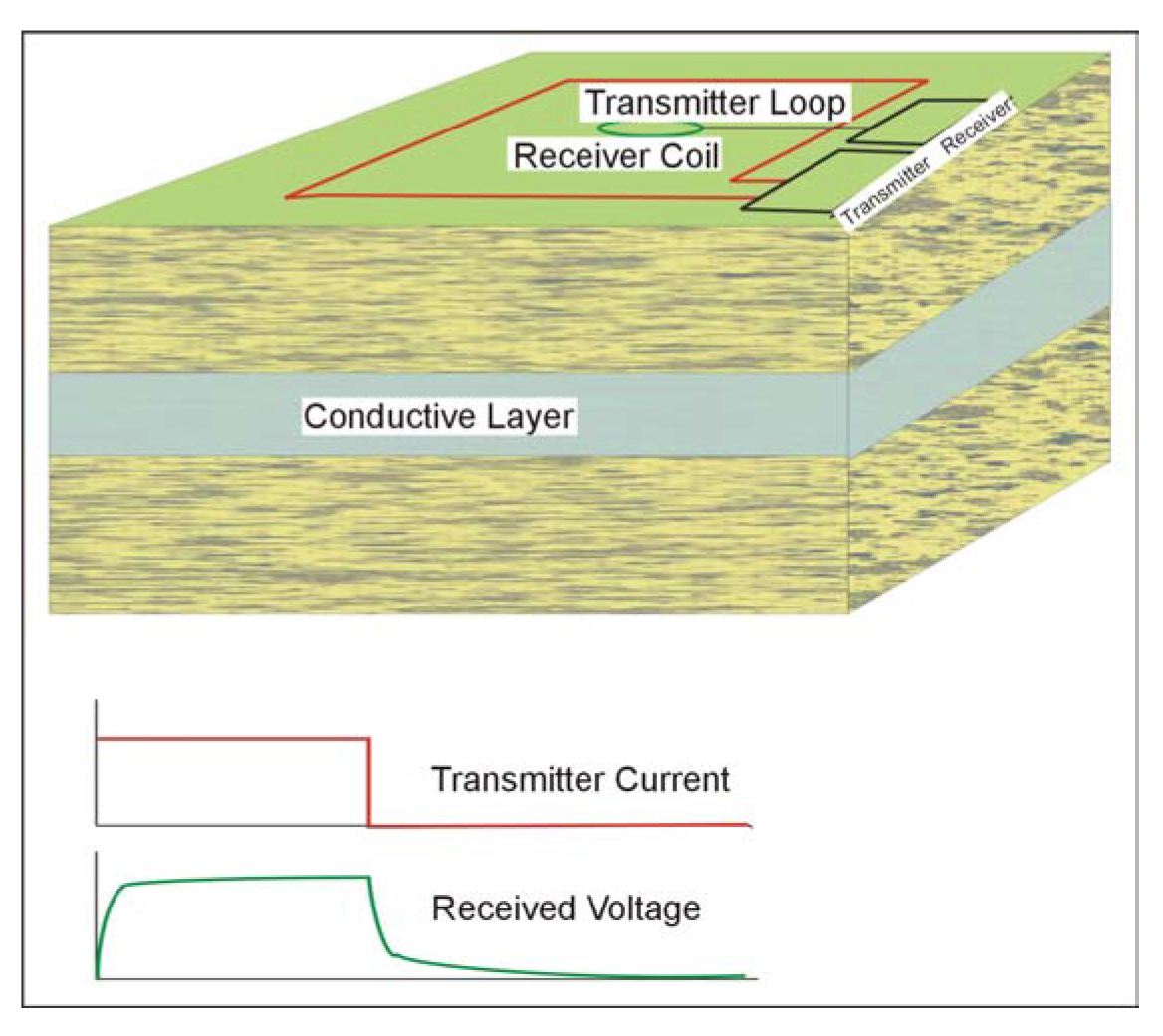
Figure 120. Time Domain Electromagnetic Soundings.

The currents in a conductive layer decay at a slower rate than those in a resistive layer. The relationship between the time after the current has turned off (delay time) and the depth and resistivity of the layers is complex, although longer delay times generally correspond to greater depths.

The voltage measured by the receiver coil does not decay instantly to zero when the current is turned off, but continues to decay for some time. This decaying voltage is caused by the decaying secondary electrical currents and the associated electromagnetic fields in the ground. The voltage measured by the receiver is then converted to resistivity. A plot is made of the measured resistivity against the delay time, as illustrated in Figure 121.

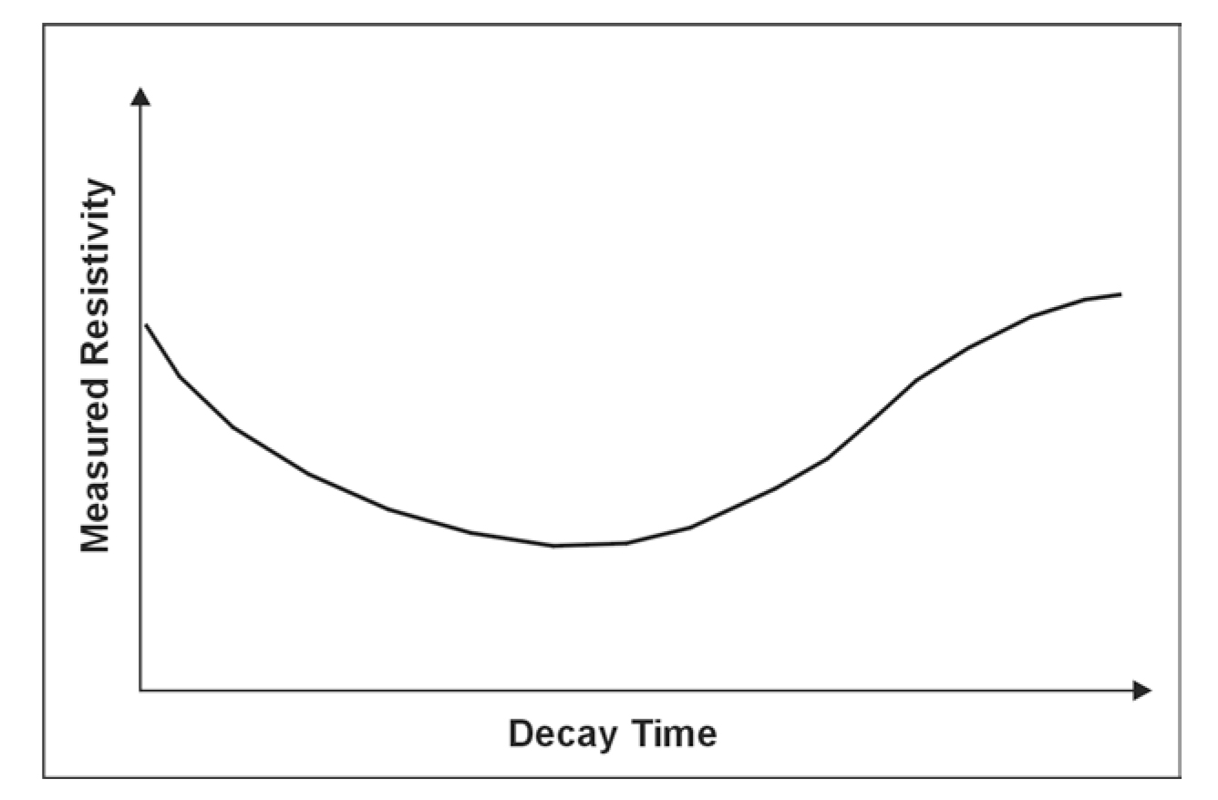
Figure 121. A Time Domain Electromagnetic Sounding curve.

The resistivity sounding curve illustrates the curve that would be obtained over three-layered ground. The near-surface layer has a higher resistivity than the middle layer. The final layer again has a higher resistivity. Figure 121 illustrates the type of curve expected over a resistive, competent limestone resting on a less competent shale.

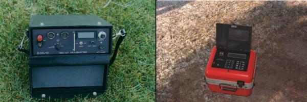
The Protem receiver and transmitter, which are used to record TDEM data, are manufactured by Geonics Ltd of Canada and are illustrated in Figure 136.

(a)         (b)

Figure 136. Protem transmitter and receiver for TDEM measurements:
(a) Protem transmitter, and (b) Protem receiver. (Geonics, Ltd.)

Data Acquisition: The field layout of the system for TDEM soundings is described above and is shown in Figure 120. Switched current is passed through the transmitter loop and the resulting voltage is measured by the receiver coil. The switching and measuring procedure is repeated many times allowing the resulting voltages to be stacked and improving the signal-to-noise ratio. Soundings are conducted at different locations until the area of interest has been covered. A sounding curve is plotted for each location showing the measured resistivity against delay time.

Data Processing: The only processing required is the possible removal of bad data points.

Data Interpretation: The sounding curves are interpreted using computer software that modifies a preliminary model input by the interpreter until the data from this model match that from the field. This process is called inversion.

Advantages: The TDEM method does not require electrodes to be inserted into the ground, as is the case with the resistivity method, and hence is an efficient method for obtaining resistivity soundings.

Limitations: Metal objects in the vicinity of the sounding site will create electromagnetic fields that will be detected by the receiver coil. This will distort the data from the ground and may produce data that are not interpretable. In addition, the interpretation assumes that the geologic layers are horizontal and have resistivities that do not change laterally. If this is not the case, the interpreted resistivities and depths may be incorrect.

Conductivity Measurements

Basic Concept: Conductivity methods can be used to map the lateral variations in bedrock conductivity (or its inverse, resistivity). Both the EM31 and EM34 can be used to record conductivity. They are designed to operate at particular frequencies and with defined transmitter and receiver coil separations such that the out-of-phase component of the received signal can be converted to apparent conductivity. These instruments use a transmitter and receiver coil, which are coplanar. Sinusoidal current, oscillating up to about 10 kHz (depending on the instrument) is passed through the transmitter coil, generating a sinusoidal electromagnetic field. This field then generates secondary sinusoidal currents in the ground, which, in turn, produce secondary electromagnetic fields that the receiver coil detects. Conductivity measurements can be recorded with the plane of the coils either parallel to the ground surface (vertical dipole mode) or orthogonal to the ground surface (horizontal dipole mode). The anomaly measured in the vertical dipole mode over a vertical, or sub-vertical conductive feature is quite distinctive and is diagnostic of that feature. Figure 128 shows the anomaly over a conductive feature (fracture zone) using an EM31 or EM34 in vertical dipole mode. In the horizontal dipole mode, only a weak anomaly would be observed, and this mode is not recommended for locating vertical conductive features.

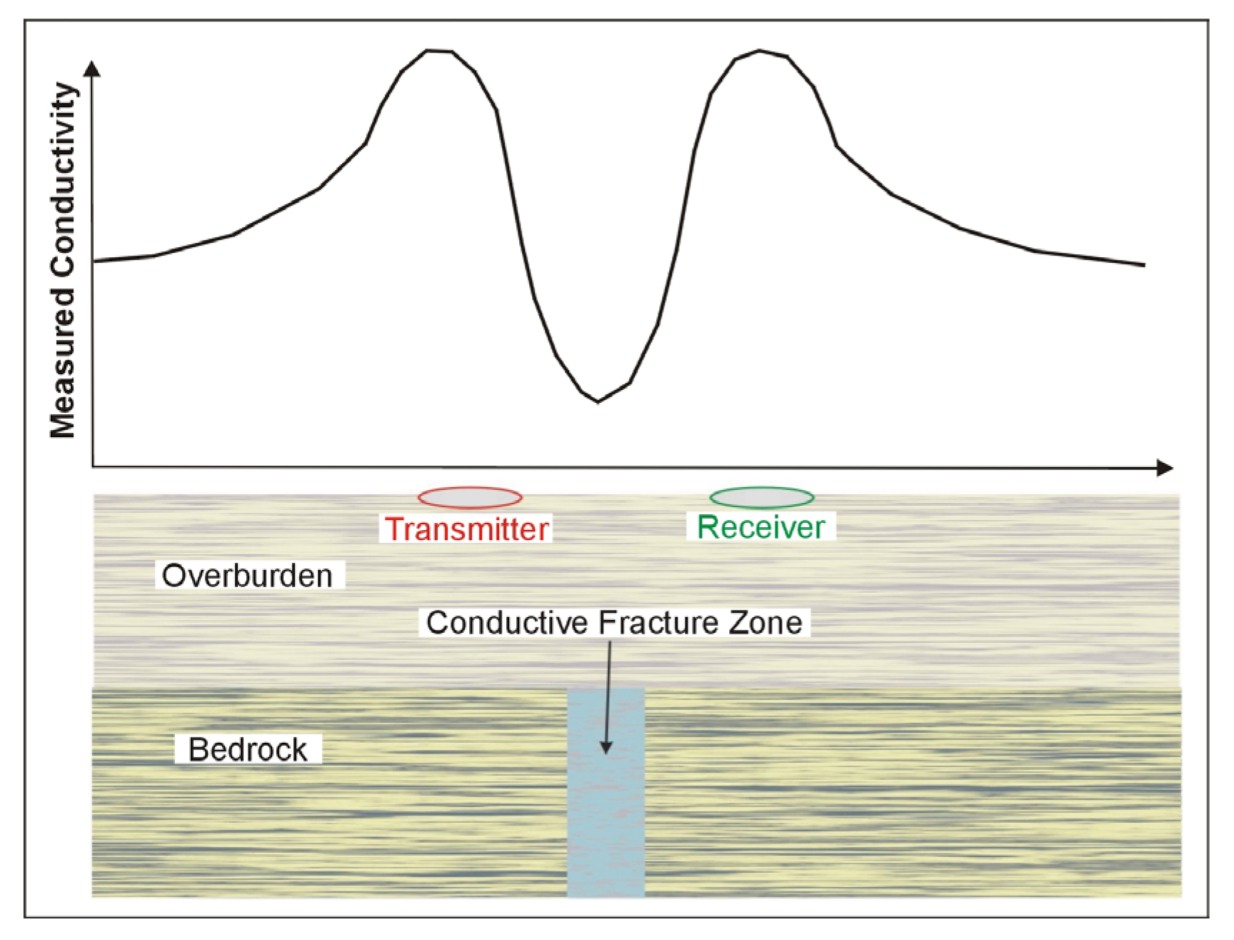
Figure 128. Anomaly from an EM31/34 used in vertical dipole mode over a conductive fracture zone.

As the conductive feature is approached, the measured conductivity increases. When the transmitter and receiver coils straddle the conductive zone, the measured conductivity values decrease, reaching a minimum when they are equally spaced about the conductive zone. This distinctive anomaly shape provides a good method for locating conductive fractures. However, this method does not provide the depth to the bedrock, and a resistivity sounding will need to be done if this is required.

Figure 183 shows the EM31 being used in the vertical dipole mode, and Figure 197 shows the EM34 being used in the horizontal dipole mode.

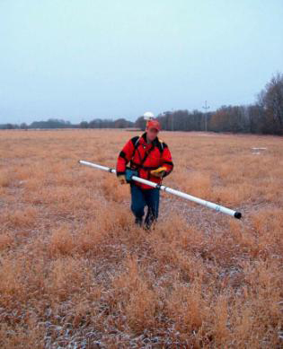
Figure 183. The EM31-MK2 Instrument. (Geonics, Ltd.)

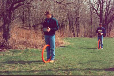
Figure 197. The EM34 being used in horizontal dipole mode. (Geonics, Ltd.)

Since, with the EM34, a cable connects the transmitter and receiver coils, their separation can be changed, thereby altering the depth of investigation. Three separations are available, 10, 20, and 40 m, providing investigation depths in the vertical dipole mode of 15, 30and 60 m.

Data Acquisition: Conductivity measurements are taken along traverses crossing the area of interest. Probably the most important decision is the particular electromagnetic system to use, since this determines the depth of investigation. The EM31 has its coils mounted in a rigid boom, and its depth of investigation in the vertical dipole mode is about 6 m. However, the EM34, as discussed above, has three discrete depths of investigation in the vertical dipole mode.

The EM31 can record data either in timed mode, i.e., every second, or when a button is pressed on the instrument (discrete mode). In timed mode, readings are taken while walking at a moderate speed. With the EM34, readings are taken while the instrument is stationary. Both the EM31 and EM34 require the station spacing be sufficient to accurately portray the shape of the resistivity curve over a conductive feature. This generally means that the station spacing should be one-fourth to one-third of the coil spacing.

Data Processing: The data are usually plotted as conductivity values against distance, and usually no processing is required.

Data Interpretation: Interpretation is mostly visual, searching for the distinctive pattern shown in Figure 128.

Advantages: Surveys with the EM31 and EM34 are generally efficient and large areas can be covered much more rapidly than with other methods, including resistivity systems.

Limitations: The EM31 provides a rapid method of measuring the ground conductivity, but only to a depth of about 6 m. The EM34 provides a much greater depth of investigation, but requires two people to operate and only takes discrete measurements. However, in spite of these limitations, the method still provides one of the most cost-effective methods of measuring ground conductivity. Neither method provides much information regarding the depth of investigation, beyond the general depths estimated for the coil separations.

These instruments (EM31 and EM34) are also influenced by both buried and aboveground metal; thus, data collected near fences and other metal objects cannot be reliably interpreted.

Rayleigh Waves Recorded with a Common Offset Array

Basic Concept: This method uses Rayleigh waves (surface waves) to detect fracture zones. Rayleigh waves have a particle motion that is counterclockwise with respect to the direction of travel. Figure 99 illustrates the particle motion for Rayleigh waves traveling in the positive X direction. In addition, the particle displacement is greatest at the ground surface near the Rayleigh wave source and decreases with depth. The effective depth of penetration is approximately one-third to one-half of the wavelength of the Rayleigh wave.

Three shot points are shown in Figure 99, labeled A, B, and C. The particle motion and displacement are shown for five depths under each shot point. For shot B, over the fracture zone, the amplitude of the Rayleigh waves is smaller than that for the other shots due to attenuation caused by the fractures and affects the measured Rayleigh waves recorded by the geophones over the fracture zone. Three parameters are usually observed. The first is an increase in the travel time of the Rayleigh waves at the fracture zone. The second is a decrease in the amplitude of the Rayleigh waves. The third parameter is reverberations (sometimes called ringing) as the fracture zone is crossed. Rayleigh wave data are recorded using a standard seismograph and geophone system.

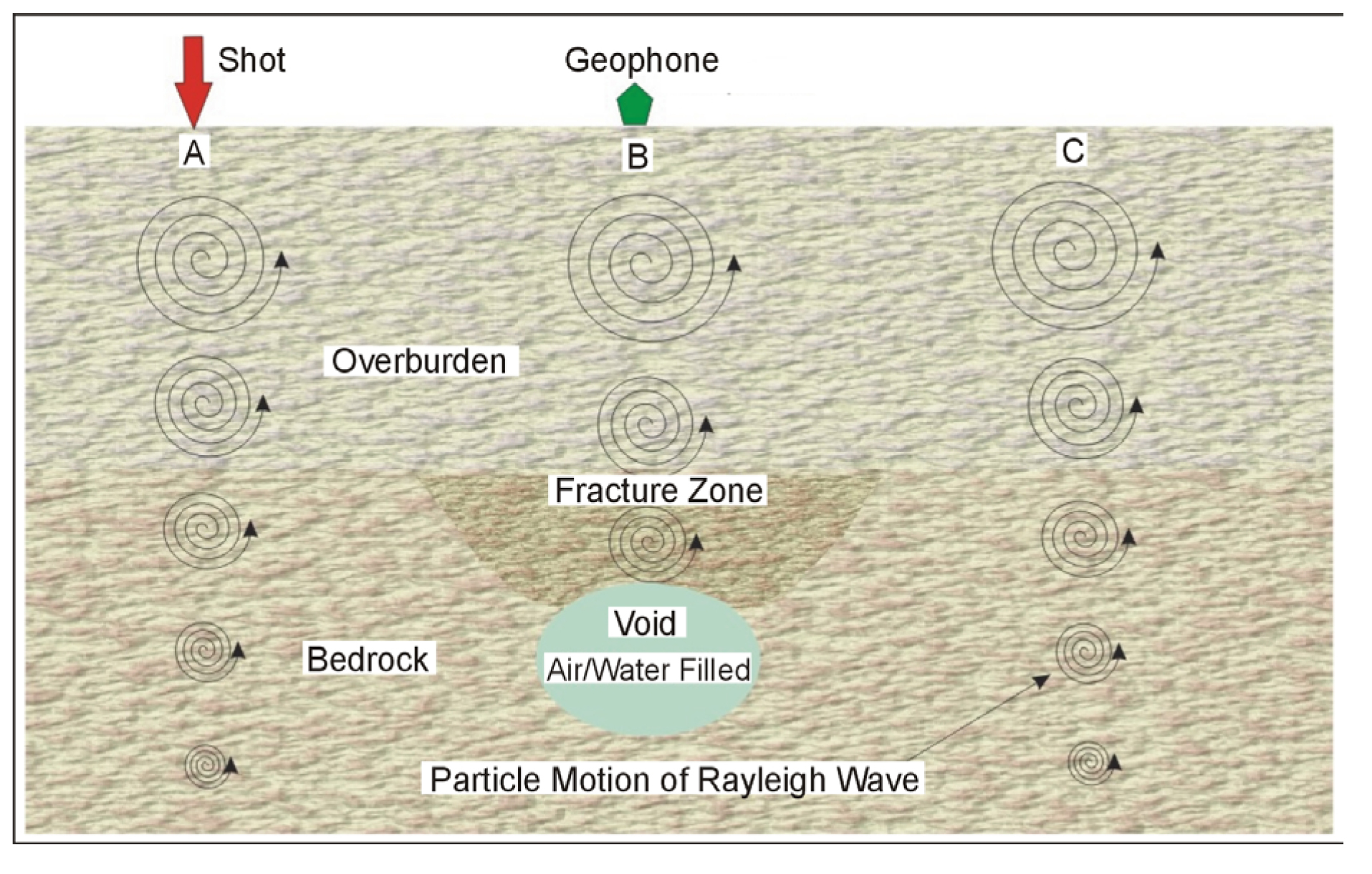
Figure 99. Rayleigh wave particle motion and displacement over a void.

Data Acquisition: Rayleigh waves are created by any impact source. For shallow investigations, a hammer is all that is needed. Data are recorded at regular intervals along a traverse using one geophone and one-shot point for each measurement, with the shot geophone distance remaining constant. The distance between the shot and geophone depends on the depth of investigation and is usually about twice the expected target depth. The interval between stations depends on the expected size of the fracture zone and the desired resolution. Generally, in order to clearly see the fracture zone, it is desirable to have at least several stations that cross this area. Data from a common offset Rayleigh wave survey over a void/fracture zone in an alluvial basin is presented in Figure 100. The geophone traces are drawn horizontally with the vertical axis being distance (shot stations).

Figure 100. Data from a Rayleigh wave survey over a void/fracture zone.

Data Processing: The data may be filtered to highlight the Rayleigh wave frequencies and are then plotted as shown on Figure 100. Spectral analysis of the individual traces can be performed that may show the lower frequencies over the fracture zone.

Data Interpretation: The data shown in Figure 100 illustrates many of the features expected over a void/fracture. The travel time to the first arrival of the Rayleigh waves is greater across the void/fracture and, in this case, is wider than the actual fractured zone. The amplitudes of the Rayleigh waves decrease as the zone is crossed. Since the records are not long enough, the ringing effect is not presented in this data.

Advantages: The field data recording is simple and efficient and requires much less effort for a given line length than seismic refraction.

Limitations: The method responds to the bulk seismic properties of the rocks and soil, which are influenced by other factors other than voids. It has a limited depth of penetration and resolution. Penetration depth is limited by the wavelengths generated by the seismic source. However, this method is faster and less costly than most other seismic methods.

Shear Wave Seismic Reflection

Basic Concept: Fracture zones can be detected using seismic shear wave reflection surveys. These surveys are conducted in much the same manner as compressional wave seismic reflection surveys, except that a shear wave source has to be used. Near-surface shear-wave seismic surveys typically employ horizontally polarized (SH) waves because they are more easily distinguished from compressional (P) waves, and they generally do not convert to P waves as readily as vertically polarized shear (SV) waves. SH waves are generated by inputting horizontal ground motion at the earth's surface by striking a fixed object with good coupling to the ground from the side. This is accomplished using some combination of mass holding the object down and spikes holding it laterally stable. There are also commercial SH sources (One such source is called the Microvib shown in Figure 95). The Microvib produces a shear wave vibration rather than an impact as with a hammer blow. Larger, truck-mounted shear wave sources are also available, one of which is called the Minivib. The Microvib is used for depths to about 100 m. Although impulse shear wave sources could be used, they have significant disadvantages compared to the Microvib source, including much lower frequencies. Shear wave impulse sources also simultaneously create some compressional waves (P-waves), which "contaminate" the shear wave data. Creating shear waves with an impulse source is much more time consuming than using the Microvib source.

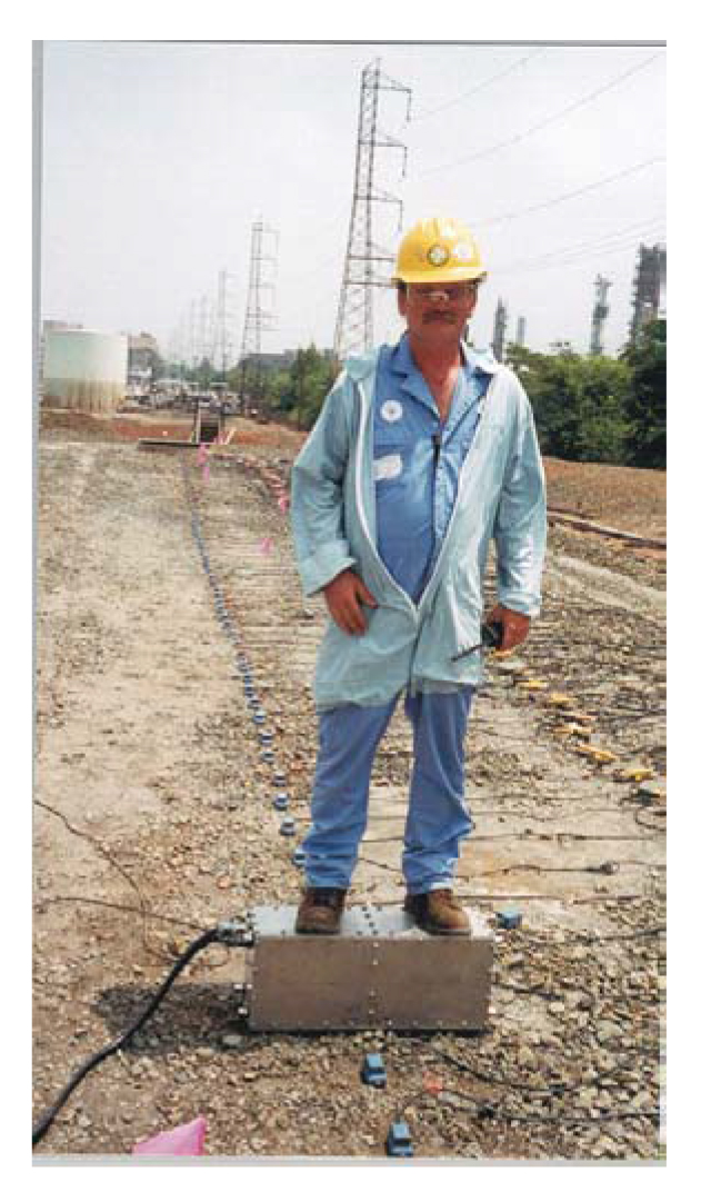
Figure 95. The Micovib shear wave generator. (Bay Geophysical)

Data Acquisition: Shear wave reflection surveys using the Microvib source are conducted much the same way as compressional wave reflection surveys using a vibroseis source. Probably the most important difference is that the geophone spacing will be smaller for an equivalent depth of investigation, since the velocity of shear waves is only about 0.6 times that of compressional waves. The geophone spacing and spread length are also dependent on the expected depth and size of the fracture zone. Another important quantity to consider is the frequency and wavelength of the shear waves. The higher the frequency, the better the resolution of detected structures. However, higher frequencies also attenuate faster and have less depth penetration.

Data Processing: The first process to be applied to shear wave data makes the data equivalent to that from an impulse source. Once this is done, standard seismic reflection processing techniques are applied. The records are sorted to gathers with a common mid-point, and various kinds of filtering and other processes are then used to refine the data. The traces for each gather are then summed to produce a single trace whose signal-to-noise ratio is much greater than the unprocessed traces. Once this procedure has been done for all of the traces, a plot is made showing the seismic traces plotted vertically against distance, called a seismic section. This plot shows the reflectors and other features imaged. Additional processing, such as migration, can also be applied to these data.

An example seismic section is shown in Figure 137 showing interpreted faults. The vertical axis is time, and the horizontal axis is distance.

Data Interpretation: Data interpretation consists mostly of visual observation of the processed seismic records. Fracture zones produce scattering of the seismic energy, resulting in less energy being reflected back to the geophones on the ground surface. Areas where the amplitude of the bedrock reflector decreases or fades out will be of interest. In addition, an increase in travel time to the bedrock reflector may also occur.

The seismic reflection method can also be used to image the vertical succession of layers, such as the weak zone produced by the shale layer in Figure 134b. Conventional data recording and processing techniques would be used, producing a seismic section showing the stratigraphy. The shale, if thick enough, would be recognized by its lower velocity. If more confirmation of the shale were required, a resistivity or TDEM sounding could be conducted. If both a low velocity and a high conductivity were obtained for the particular horizon, the chances of it being a shale layer would be substantially increased.

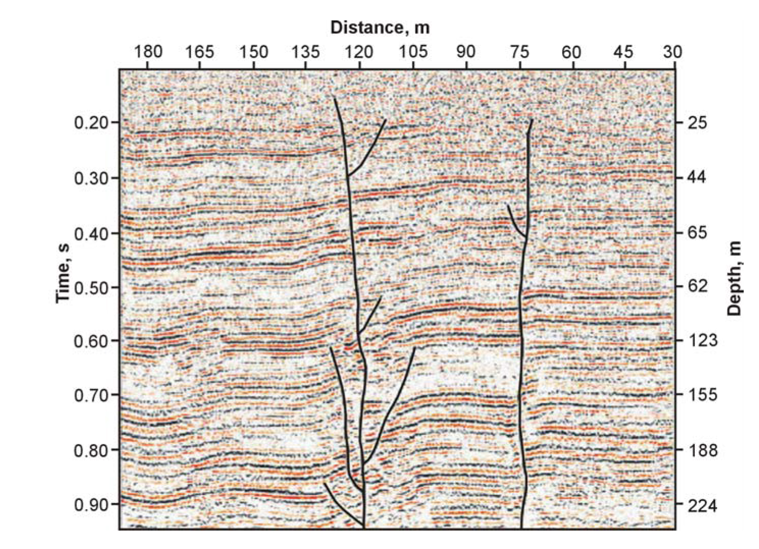
Figure 137. Example seismic section showing interpreted faults. (Bay Geophysical)

Figure 134a. Bedrock surface formed from a series of dipping layers.

Figure 134b. Weak zone comprising a thin, competent limestone layer overlying a weak shale layer.

Advantages: The reflection seismic method generally proved the best resolution (except for GPR) for structural information

Limitations: The seismic reflection method is quite labor intensive, and significant data processing is required. This is one of the more expensive geophysical methods. In addition, any local vibration source, including industrial areas and road traffic, may produce noisy data.

Seismic Refraction

Basic Concept: The seismic refraction method can be used to locate fractures and weak zones. The method requires a seismic energy source, usually a hammer for depths less than 30 m and black powder seismic guns ges for depths over 30 m. The seismic waves then penetrate the overburden and refract along the bedrock surface. While they are traveling along this surface, they continually radiate seismic waves back to the ground surface. These are then detected by geophones placed on the ground surface. Both compressional waves and shear waves can be used in the seismic refraction method, although compressional waves are most commonly used. Figure 114a shows the layout of the instrument, the main seismic waves involved, and the resulting time-distance graph.

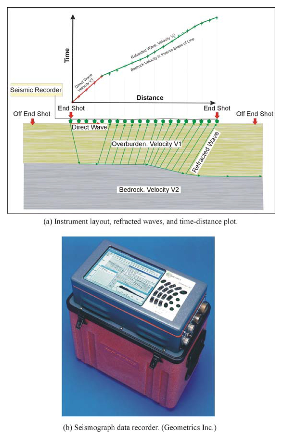
Figure 114. Seismic Refraction: field set up and data recorder.

Surveys for fracture zones are somewhat different from the more conventional application of the seismic refraction method, which is mapping bedrock topography, as illustrated in Figure 114. Bedrock fracture zones are recognized from the character of the first signal arrivals at the geophones. Fracture zones attenuate the signal and can cause time shifts as illustrated in Figure 94. In this case, the amplitudes of the traces from geophones 2 and 3 are attenuated.

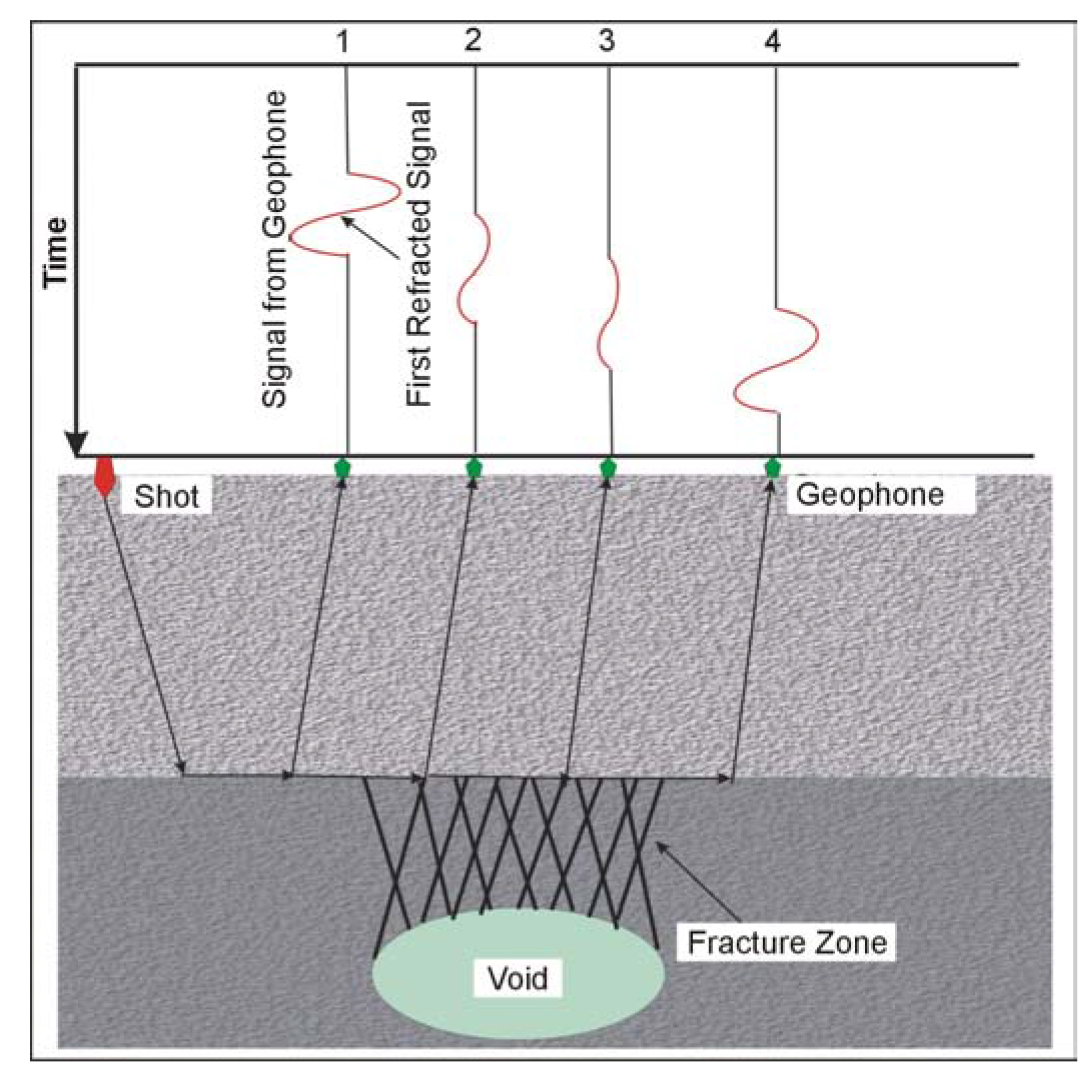
Figure 94. Seismic refraction across a fracture zone.

In addition to compressional wave surveys for fracture detection, shear wave surveys can also be used. If a shear wave is oscillating at right angles to its direction of travel, then its amplitude will be severely attenuated as it passes a fracture or fracture zone. However, if the shear wave is oscillating in the direction of travel, then the fracture zone has little effect.

Data Acquisition: The design of a compressional wave seismic refraction survey requires a good understanding of the expected bedrock and overburden. With this knowledge, velocities can be assigned to these features and a pre-survey model developed that will show the parameters of the seismic spread best suited for a successful survey. These parameters include the length of the geophone spread, the spacing between the geophones, and the expected first break arrival times at each of the geophones. Knowing the expected first break arrival times is also helpful in the field, where field arrival times that correspond fairly well to expected times help to confirm that the spread layout has been appropriately planned, and that the target layer (bedrock) is being imaged. Surveys will be conducted by recording contiguous seismic spreads along traverses crossing the area of interest.

Data Processing: In order to interpret seismic refraction data for depths, the first arrival times of the refracted rays have to be picked. Once this is done these times are then input to interpretation software. If the data is to be used for locating fracture zones then it has to be plotted in order for the amplitudes of the first arrivals to be compared.

Data Interpretation: Interpretation of seismic refraction data for fracture or weak zones is mostly visual. The geophone traces have to be plotted for each seismic spread and viewed for areas of amplitude attenuation and possibly an increase in the time to the first arrival if the fracture zone is accompanied by a bedrock depression. The seismic refraction method could not be used to image the shale layer underlying the limestone illustrated in Figure 134b. This is because the shale will probably have a lower velocity than the limestone and will not produce refractions, and would not, therefore, be observed by a seismic refraction survey.

Advantages: The seismic refraction method, using amplitude changes to locate fractures, usually provides good resolution for any observed fractures.

Limitations: It is clearly important that the seismic waves refract from the bedrock layer of interest. Usually this will be easily recognized. However, if refracting layers lie above the bedrock surface, these must be recognized. If the local geology is known from previous surveys or drill holes, a pre survey model will assist in identifying the travel times at which a seismic arrival from the bedrock is expected. If this is not known, a conventional seismic spread, as shown in Figure 114a, should be applied and interpreted.

If the water table is in the overburden and close to the bedrock, this may obscure the water table arrivals, since bedrock has a higher velocity than saturated soils. In some cases, water above the bedrock may remove the velocity contrast between the unsaturated overburden and the bedrock.

Local noise, for example traffic, may obscure the refractions from the bedrock. This can be overcome by using larger impact sources or by repeating the impact at a common shot point several times and stacking the received signals. If noise is still a problem, a larger energy source may be required. In addition, since some of the noise travels as airwaves, covering the geophones with sound absorbing material may also help to dampen the received noise.

Ground Penetrating Radar

Basic Concept: Ground Penetrating Radar (GPR) can be used provided the conditions are appropriate for the method. For the method to work, the bedrock and fracture or weak zone must provide a contrast in dielectric properties from those of the overburden. Ideal conditions for this method are a dry sandy overburden. If clay occurs in the overburden, or if it is saturated, penetration may be limited. However, in ideal conditions, the method may penetrate to depths of 15 m.

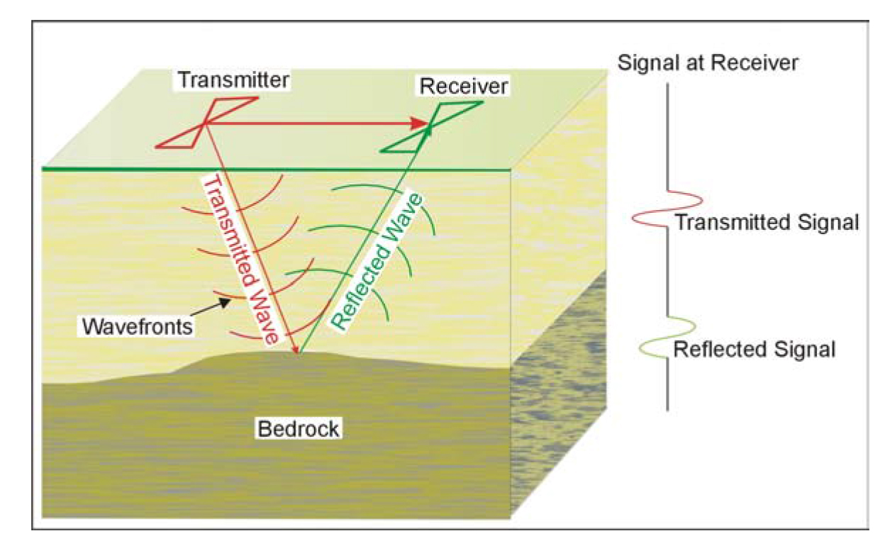
Figure 111. Ground Penetrating Radar system.

The GPR instrument consists of a recorder and a transmitting and receiving antenna. Different antennae provide different frequencies. Lower frequencies provide greater depth penetration but lower resolution. Figure 111 provides a drawing illustrating the GPR system. The transmitter provides high-frequency electromagnetic signals that penetrate the ground and are reflected from objects and boundaries providing a different dielectric constant from that of the overburden. The reflected waves are detected by the receiver and stored in memory.

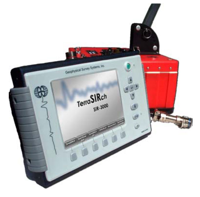
Figure 138. Ground Penetrating Radar equipment. (Geophysical Survey Systems, Inc.)

Figure 138 shows the data recording and system control for a GPR instrument. Any antenna supported by this instrument can be attached and used to collect data. Figure 139 shows a 250 MHz antenna being used in a field survey.

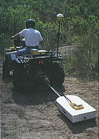
Figure 139. A 250 MHz antenna being used in a field survey. (MALA GeoSCiences, Inc.)

Data Acquisition: GPR surveys are conducted by pulling the antenna across the ground surface at a normal walking pace. The recorder stores the data, as well as presenting an image of the recorded data on a screen.

Data Processing: It is possible to process the data, much like the processing done on single- channel reflection seismic data. Techniques that can be applied include distance normalization, horizontal scaling (stacking), horizontal and vertical filtering, velocity corrections, and migration. However, depending on the data quality, this may not be necessary since the field records may be all that is needed to observe the fracture zone.

Data Interpretation: Interpretation of GPR data for fractures may involve searching for reflectors if the fractures are sub-horizontal to zones where the signal coherence is lost due to scattering of the waves caused by near-vertical fracture zones. In addition, if the fracture zone is saturated, this may attenuate the GPR signal, causing decreased amplitudes over this zone.

To calculate the depth to the feature of interest, the speed of the GPR signal in the soil at the site needs to be obtained. This can be estimated from textbook speeds for typical soil types, or it can be obtained in the field by conducting a small traverse across a buried feature whose depth is known.

Figure 129 presents a GPR profile over a fracture zone. In this case, the bedrock is quite shallow, and the fractures can be seen in a local roadcut. However, it does show the potential of the method if conditions are appropriate. In this case the fracture zones are sub-horizontal and is recognized as a reflector.

G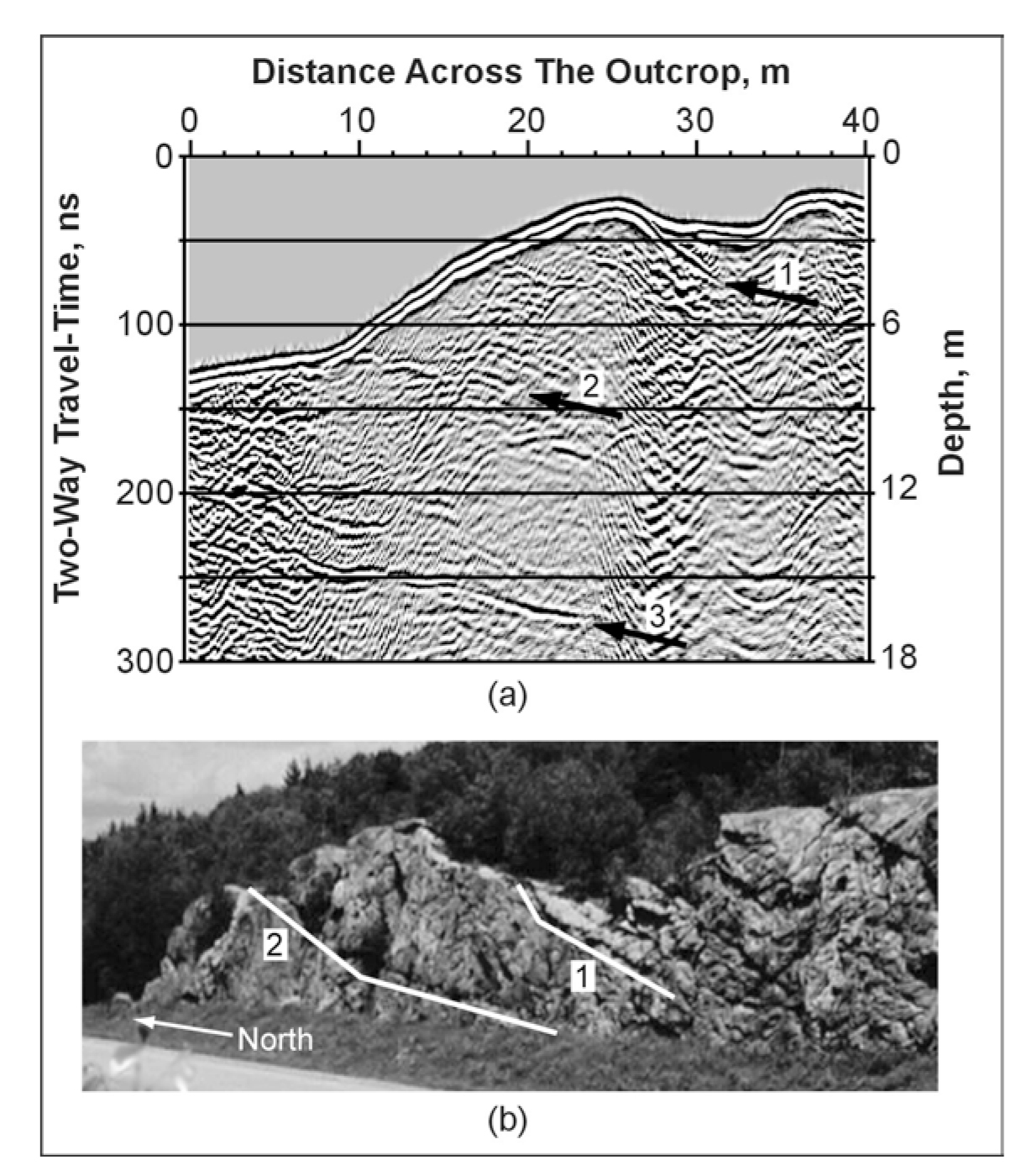

Figure 129. Ground Penetrating Radar data illustrating a section over a fracture zone. (Lane, 2000)

Advantages: The method is fairly rapid in the field and since the data is displayed in real time, fractures may be observed when the data is recorded. This may allow parallel lines to be surveyed in order to map the extent of the fracture.

Limitations: Probably the most limiting factor for GPR surveys is that their success is very site specific and depends on having a contrast in the dielectric properties of the target compared to the host overburden, along with sufficient depth penetration to reach the target. However, it is likely in many cases that the bedrock will provide a dielectric contrast with the overburden, making depth of penetration probably the most important factor.

Very Low Frequency Electromagnetic Surveys

Basic Concept: The Very Low Frequency (VLF) method is an electromagnetic technique that uses powerful military transmitters producing electromagnetic fields with frequencies between 15 and 40 kHz. The VLF method can be used to locate saturated (conductive) near-vertical zones in which the primary field induces current flow. The field radiated from a VLF transmitter over a uniform or horizontally layered ground consists of a vertical electrical field component and a horizontal magnetic field component, each perpendicular to the direction of propagation. Because the source of the field is usually many kilometers from the survey area, the EM wave approximates a plane wave.

VLF is often used in two modes measuring tilt angle and resistivity. For tilt angle measurements, magnetic field coupling with the fracture zone is important. Therefore, the VLF transmitter should be located along the strike of the target. The depth of investigation depends on the frequency used and the resistivity of the host medium. It can vary from a few meters to over 100 m.

Measuring resistivity with the VLF equipment requires measuring the electric field with two electrodes connected to the control unit with a wire. For resistivity measurements, the electrical field coupling with the fracture zone is important. Therefore, the VLF transmitter should be located in a direction perpendicular to the target.

A VLF instrument is shown in Figure 140. This instrument can also provide its own electromagnetic field source.

Data Acquisition: As mentioned above, it is preferable to have the transmitter located along strike when measuring tilt angles and perpendicular to strike when measuring resistivity. Measurements are made while traversing across the feature or area of interest. A conductive feature produces an anomaly similar to that shown in Figure 141.

The data are plotted as a graph of magnetic field component against distance, similar to that shown in Figure 141.

Data Processing: Usually minimal processing is done to the data, although various spatial filters can be applied to remove noise.

Data Interpretation: Interpretation is mostly visual searching for anomalies.

The conductive feature shown in Figure 141 produces a tilt angle anomaly that looks similar to a sinusoid. The top of the fracture is centered at the inflection point of the anomaly.

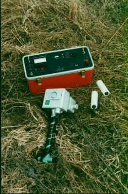
Figure 140. Very Low Frequency (VLF) instrument. (Geonics Ltd.)

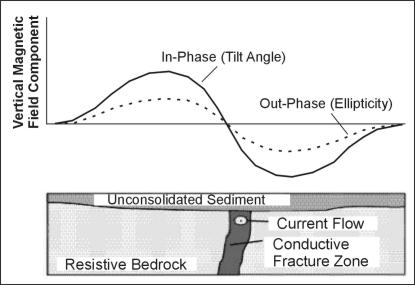
Figure 141. Very Low Frequency (VLF) anomaly over a vertical conductor.

Advantages: The main advantage of the VLF method is that it is a rapid and inexpensive method.

Limitations: The VLF method is somewhat restrictive if the military VLF transmitters are to be used in that it works best for specific orientations of the fracture relative to the transmitter location, as discussed above. In addition, sometimes the VLF transmitter station desired is not broadcasting and cannot be used.

Exploration depths will be limited if the ground is electrically conductive. In addition, anomalies can be created by other geologic conditions unrelated to fractures such as changes in overburden thickness or conductivity.

Generally, methods using active sources (EM31, EM34) are preferred to the VLF method since these have no target orientation restrictions. Because these are active methods, they do not rely on other transmitters to produce the required electromagnetic field.

Borehole Televiewers (Optical & Acoustic)

Optical and acoustic televiewers are used for imaging stratigraphic and concrete features and for measuring fracture orientation and distribution (Figure 142). Images are based on direct optical mapping or on the amplitude and travel time of an ultrasonic beam, reflected from the borehole wall. From televiewer imaging, fractures and bedding planes can be mapped over the length of the borehole. These planar features can be tabulated, analyzed, and expressed statistically in order to identify subsurface fracture zones, weak zones, and zones of subsurface flow.

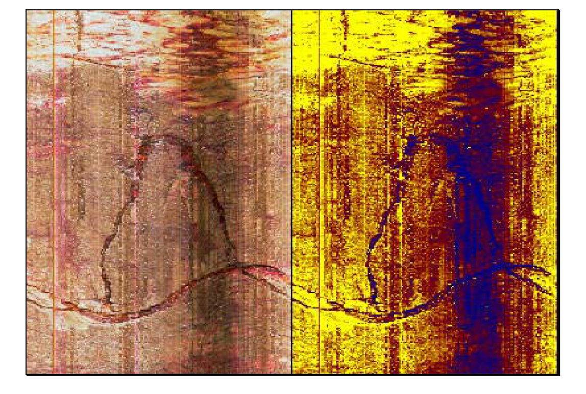
Figure 142. Examples of typical borehole images, optical and acoustic. (Layne Christensen, Colog)

Basic Concept: Televiewer probes provide images of the inside of boreholes by capturing a layer of several samples around the circumference of the hole and stacking the layers to reproduce a full, in-situ, oriented image of the borehole wall.

A televiewer log can be thought of as a cylinder that is opened along the north side. Planer features that intersect the borehole appear to be sinusoids on the unwrapped image (Figure 143). Calculation of the dip direction and dip angle of a fracture requires the vertical intercept h and the direction of the dip from the televiewer log, and the diameter d of the borehole from the caliper log or known bore diameter. The angle of dip is equal to the arc tangent of h/d, and the dip direction is picked at the trough of the sinusoid.

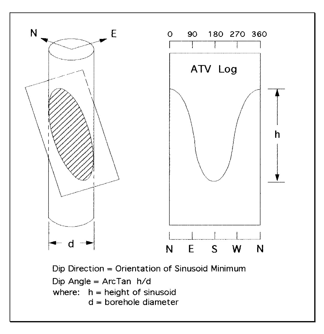
Figure 143. Projection of a planar intersection with a cylindrical borehole. (Layne Christensen, Colog)

Data Acquisition: To record a televiewer log, the appropriate probe is lowered slowly into a borehole, with depth being precisely recorded with regard to the data-conducting wireline. As the probe proceeds downhole, optical images or acoustic reflection parameters are digitized and displayed in real-time. Probes are carefully centralized within the borehole, and they record the azimuth and tilt of the borehole, along with image information. All data is recorded directly to a computer hard-drive. These data files and the relatively large but can be easily transferred via LAN, high-speed internet, or CD-ROM. The Optical televiewer is optimized when the borehole is air or clear-fluid filled, while acoustic televiewer requires the presence of fluid regardless of its clarity.

Data Processing: Oriented borehole images are picked manually, using software, searching for sinusoidal features. Such features correspond to planar intersections with the borehole (Figure 143). By measuring the height, direction, and dip of each feature, statistical summaries such as stereonet and rose diagrams can be presented (Figure 144).

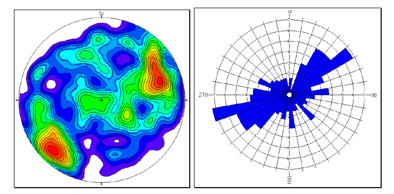
Figure 144. Statistical representations of fracture orientations. (Layne Christensen, Colog)

Data Interpretation: Dominant trends that present themselves in the orientation of planar features are directly related to fluid flow patterns, slope failure planes, and zones of weak or unstable subsurface. Depths to stable or unstable layers can be established.

Advantages: Borehole televiewer imaging provides information about the subsurface geology as it exists, in-situ, under natural temperature and pressure conditions. Unlike drilled core, imaging produces 100% recovery, with highly accurate depth and orientation control. Borehole televiewer imaging is rapid, and considerably less expensive than the recovery, transport, analysis, and storage of oriented core.

Limitations: Optical imaging required an optically transparent medium between the probe and the borehole wall, while acoustic imaging requires a liquid medium. Televiewer logs should be included in a suite of logs that can provide an array of subsurface information, and specific core samples may still be recovered for lab analysis. Image orientation can be affected by magnetic material, including rebar, within the near vicinity of the borehole.