This section discusses the determination of bedrock depths for materials source areas, foundations, mapping bedrock topography and mapping bedrock structure. The determination of bedrock depths is common to each of these topics, since bedrock topography is simply the lateral changes in bedrock depths. Bedrock structure is related more to fractures, faulting, and other features, although bedrock depth may also be important. The section is broadly divided into two parts with the first part describing the methods used to map bedrock depths. The second part concentrates on the methods that can be used to map fractures.

Unfortunately, no geophysical method, except possibly Ground Penetrating Radar under ideal conditions, can map fine/detailed structure internal to the bedrock. Generally, only successively deeper layers beneath the bedrock can be mapped geophysically. However, geophysical methods can be used to map fracturing, faulting, locate voids, and for other targets as described in other sections of this web manual.

Many of the methods used to map bedrock topography can also be used to locate fractures; hence, the basic theory of the method is common to both applications. It is, therefore, convenient to divide this section into two main parts. The first part discusses the basic theory of each method as well as presents its application to mapping bedrock topography and providing bedrock depths. The second part of this section will focus on the application of the techniques to locate fractures but will not describe the basic theory of each method, since these are described in the first section. Exceptions to this will be methods that are used only for detecting fractures but are not used to find bedrock depths and are not described in the first section. Finally, a brief discussion of the use of geophysical methods to map faults is given at the end of this section.

Methods to Map Bedrock Depths and Topography

Determining bedrock depths and topography is commonly done using geophysical methods. As with all geophysical methods, estimating the physical properties of the geologic section prior to conducting a survey is important in determining the best method to use. The estimated depth to the bedrock is also an important criterion, since some methods may not be able to penetrate to the required depths.

Determining bedrock depths and topography are somewhat different in that mapping the topography of the bedrock does not necessarily imply that its depth is known. However, usually, its depth can be found, and the topographic profile can be converted to a depth profile. There are several geophysical methods that are used to find depths to bedrock and map bedrock topography. These methods are listed below.

1. Ground Penetrating Radar (GPR).
2. Seismic Refraction.
3. Seismic Reflection.
4. Resistivity methods.
5. Time Domain Electromagnetic Soundings (TDEM).
6. Conductivity measurements using the EM31 and EM34.
7. Spectral Analysis of Surface Waves (SASW).
8. Analyzing acoustic noise using the SeisOpt software.
9. Gravity.

Ground Penetrating Radar (GPR)

Basic Concept: Ground-Penetrating Radar can be used where the bedrock is expected to be relatively shallow, and the overburden is unsaturated and contains little clay or silt. If these conditions exist, then penetration depths may be a few meters to a few tens of meters. The GPR instrument consists of a recorder and a transmitting and receiving antenna. Different antennas provide different frequencies. Lower frequencies provide greater depth penetration but lower resolution. Figure 111 illustrates the GPR system. The transmitter provides the high-frequency electromagnetic signals that penetrate the ground and are reflected from objects and boundaries, providing a different dielectric constant exists from that of the overburden. The reflected waves are detected by the receiver and stored in memory.

Figure 112 shows typical GPR equipment that includes the display and controls for the equipment.

Figure 113 shows a 100 MHz antenna being pulled across the ground as the survey is conducted. This is a fairly low-frequency antenna and can provide penetration to about 20 m.

Data Acquisition: GPR surveys are conducted by pulling the antenna across the ground surface at a normal walking pace, as shown in Figure 113. The recorder stores the data, as well as presenting an image of the recorded data on a screen.

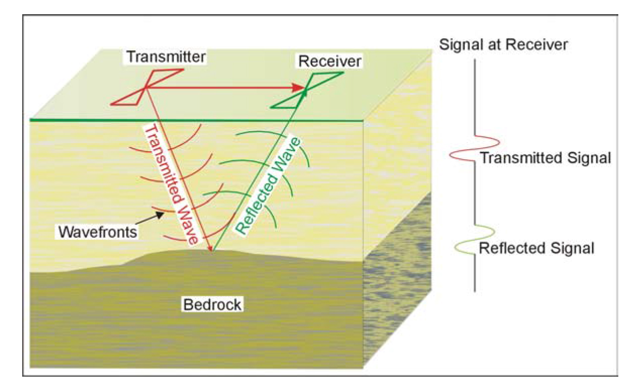
Figure 111. Ground Penetrating Radar system.

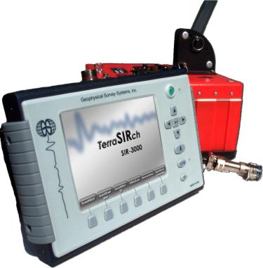
Figure 112. Ground Penetrating Radar instrument. (Geophysical Survey Systems, Inc.)

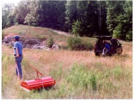
Figure 113. GPR antenna (100 MHz) used in a survey. (MALA GeoScience USA, Inc.)

Data Processing: The data are processed much like the processing done on single channel reflection seismic data. Processes such as distance normalization, horizontal scaling (stacking), vertical and horizontal filtering, velocity corrections, and migration can all be done. However, depending on the data quality, it may not be necessary to process the data since the field records may be all that is needed to observe the bedrock.

Data Interpretation: In order to calculate the depth to the bedrock, the speed of the GPR signal in the soil at the site needs to be obtained. This can be estimated from propogation speeds for typical soil types or it can be obtained in the field by conducting a small traverse across a buried feature whose depth is known.

Advantages: GPR is a relatively fast method and presents results as the survey progresses. Different antenna can easily be attached and tested if the resolution or depth penetration is insufficient.

Limitations: Probably the most limiting factor for GPR surveys is that their success is very site specific, and depends on having a contrast in the dielectric properties of the target compared to the host overburden. Clearly sufficient depth penetration to reach the target is needed. Penetration depends on the frequency of the antenna, the conductivity of the overburden, and whether clay is present in the overburden. Also, if a low-frequency antenna is used, then the resolution of targets is less than with a high-frequency antenna. In addition, with low-frequency antennas, which are usually not shielded, GPR energy radiates in all directions. Thus, reflections occur from local objects either on the ground surface or above the ground, such as power lines and buildings. For surveys under bridges, the bridge deck may provide a reflection. It may be possible to separate the reflection from the bridge deck from the reflection from the bedrock, providing these two reflection times are significantly different.

Seismic Refraction

Basic Concept: Seismic refraction is one of the most commonly used methods to determine bedrock depths, especially for depths of less than 30 m. The method requires a seismic energy source, usually sledgehammers for depths of 30 m or less, and weight drops and black powder seismic guns for depths over 30 m. The seismic waves produced by the energy source penetrate the overburden and refract along the bedrock surface. While they are traveling along this surface, they continually radiate seismic waves back to the ground surface. These are detected by geophones placed on the ground surface. Both compressional waves (P-waves) and shear waves (S-waves) can be used in the seismic refraction method, although compressional waves are most commonly used. Figure 114a shows the layout of the instrument, the main seismic waves involved, and the resulting time distance graph. A typical seismic recorder is shown in Figure 114b. The method can be used for up to about four layers. However, each layer has to have a higher velocity than the overlaying layer.

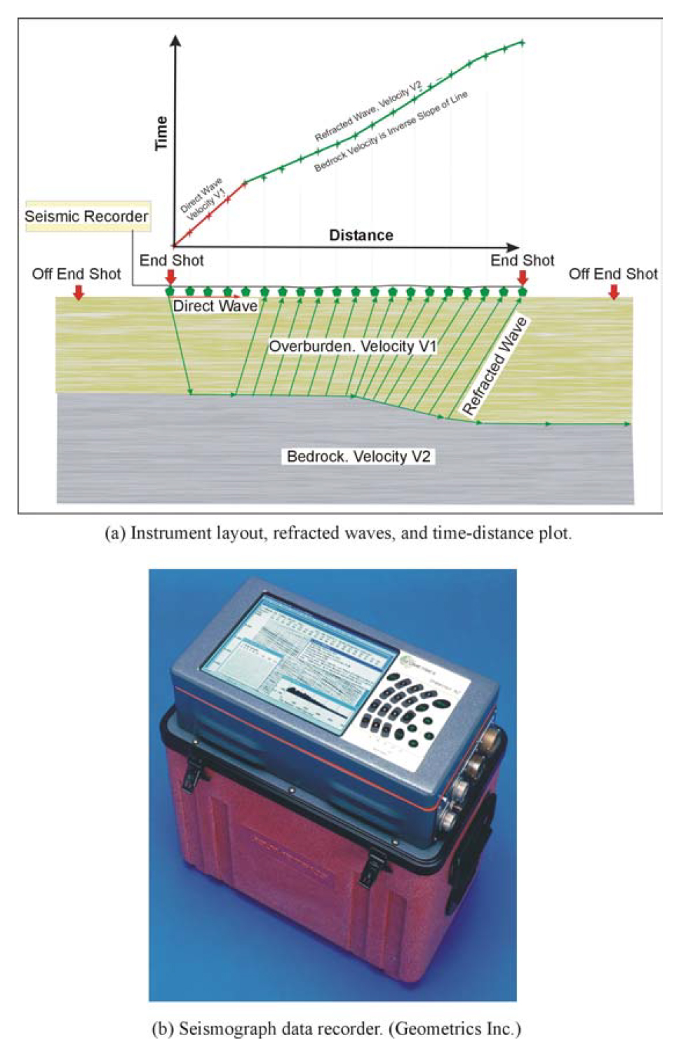
Figure 114. Seismic Refraction: field set up and data recorder.

Data Acquisition: The design of a seismic refraction survey requires a good understanding of the expected bedrock velocity and depth and overburden velocity. With this knowledge, velocities can be assigned to these features and a model developed that will show the parameters of the seismic spread best suited for a successful survey. These parameters include the length of the geophone spread, the spacing between the geophones, the expected first break arrival times at each of the geophones, and the best locations for the off-end shots. Knowing the expected first break arrival times is also helpful in the field, where field arrival times that correspond fairly well to expected times help to confirm that the spread layout has been appropriately planned, and that the target layer is being imaged.

Data Processing: The first step in processing/interpreting refraction seismic data is to pick the arrival times of the earliest seismic signal, called first break picking. A plot is then made showing the arrival times against the distance between the shot and geophone. This is called a time-distance graph. An example of such a graph for two-layered ground (overburden and refractor) is shown in Figure 114a.

The red portion of the time distance plot in Figure 114a shows the waves arriving at the geophones directly from the shot. These waves arrive before the refracted waves. The green portion of the graph shows the waves that arrive ahead of the direct arrivals. These waves have traveled a sufficient distance along the higher speed refractor (bedrock) to overtake the direct wave arrivals.

Data Interpretation: Several methods of refraction interpretation are used. In recent years, seismic refraction tomography (SRT) has gained popularity and is now the most common method used for interpreting refraction data. The main benefit with SRT is that it allows for obtaining a picture of the velocity distribution in the subsurface highlighting continuous lateral and vertical changes in velocity rather than assuming a layered model.

The SRT technique involves an automated search for the minimum deviation between the measurements made on the ground and the "virtual" measurements of a synthetic model through an iterative computer process. An example of a SRT velocity model is shown in Figure 114c.

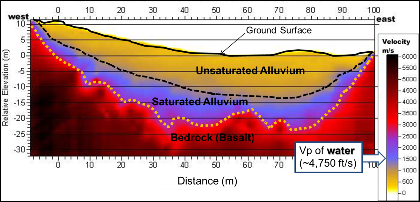
Figure 114c. Bedrock and water table mapping (Image courtesy of USGS).

Another popular method is the Generalized Reciprocal Method (GRM) that is also described in detail in Part 2 Geophysical Methods, Theory and Discussion. A brief, and simplified, description of the GRM method is presented below. Figure 115 shows the basic rays used for this interpretation.

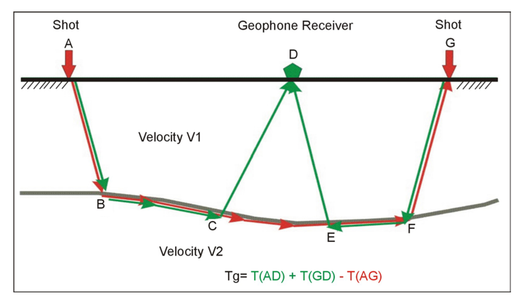
Figure 115. Basic Generalized Reciprocal method interpretation.

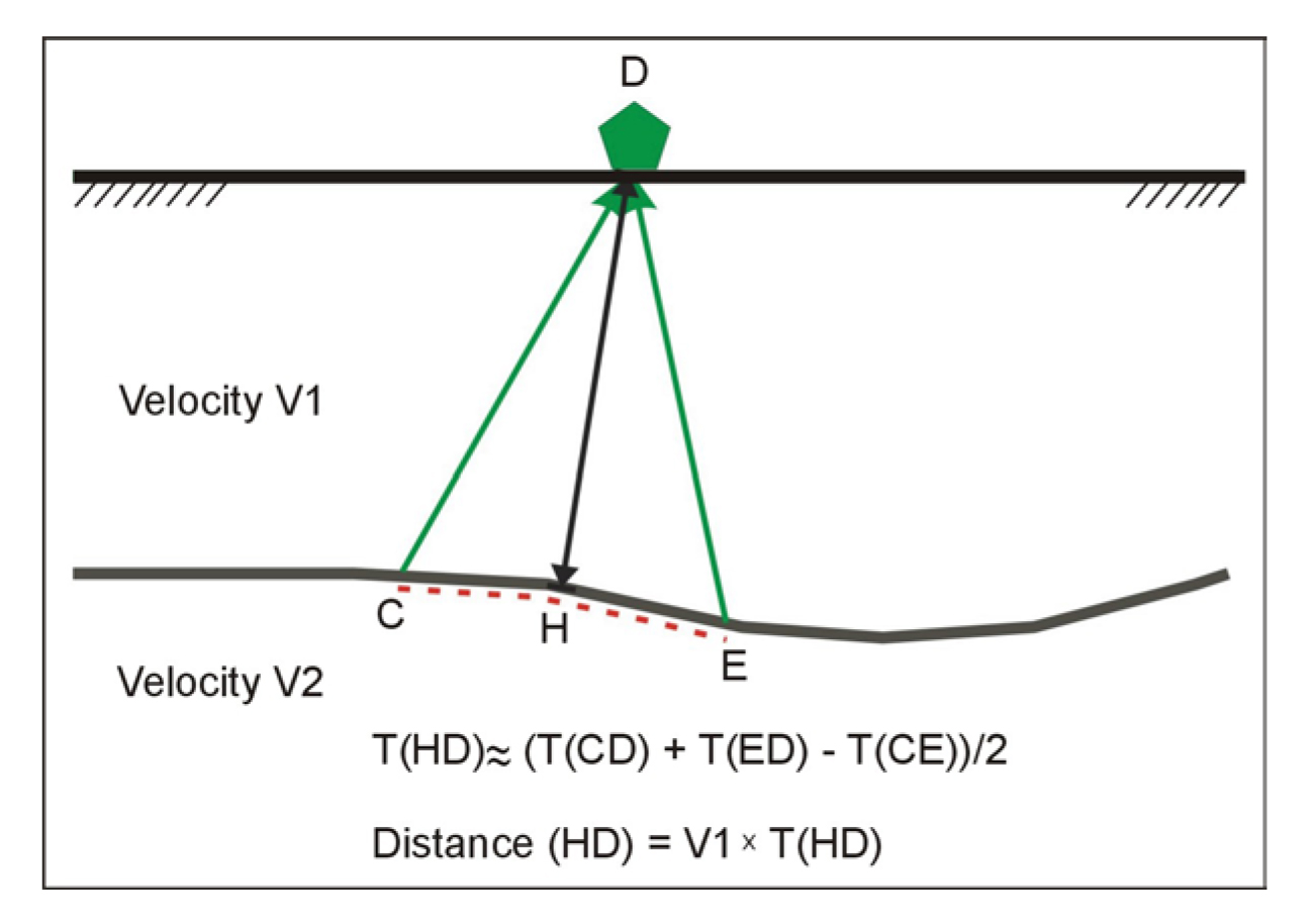
Figure 116. Generalized Reciprocal method interpretation.

The objective is to find the depth to the bedrock under the geophone at D. This is done using the following simple calculations. The travel times from the shots at A and G to the geophone at D are added together: T1= T(AD) + T(GD). The travel time from the shot at A to the geophone at G is then subtracted from T1. Figure 116 shows the remaining waves after the above calculations have been performed. These are the travel times from C to D added to the travel times from E to D subtracting the travel time from C to E. The sum of these travel times can be shown to be approximately the travel time from the bedrock at H to the geophone at D. Since the velocity of the overburden layer can be found from the time distance graph, the distance from H to D can be found giving the bedrock depth.

An example of the results from a seismic refraction survey is presented in Figure 117. The upper Figure shows the travel time graph, illustrating the time that the seismic waves take from the shot to each geophone. The second graph presents the interpreted seismic velocities, and the third graph shows the interpreted bedrock section.

Advantages: Refraction seismic is generally very effective at determining bedrock depths since bedrock usually has a higher velocity than the overburden. In addition, the method can provide fairly detailed lateral variations in depth since the depth beneath each geophone can be determined.

Limitations: Probably the most restrictive limitation is that each of the successively deeper layer must have a higher velocity than the shallower layer. However, for determining bedrock depths, this is probably in most cases not a significant limitation since, as mentioned above, the bedrock usually has a higher velocity than the overburden.

If the water table is in the overburden and close to the bedrock, this may obscure the water table arrivals since bedrock has a higher velocity than saturated soils. This may result in a false interpretation of the bedrock depth.

Local noise, for example, traffic, may obscure the refractions from the bedrock. This can be overcome by using larger impact sources or by repeating the impact at a common shot point several times and stacking the received signals. If noise is still a problem, a larger energy source may be required. In addition, since some of the noise travels as airwaves, covering the geophones with sound absorbing material may also help to dampen the received noise.

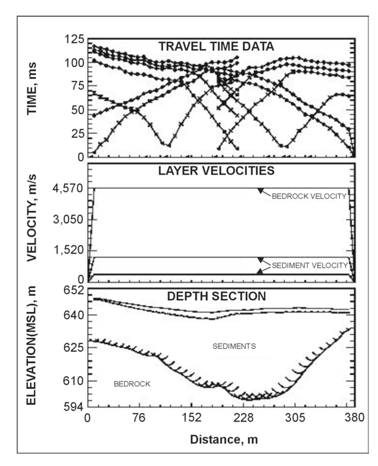
Figure 117. Example of a SeismicRrefraction interpretation.

Seismic Reflection

Basic Concept: Seismic reflection involves using a surface seismic source to create a seismic wave, which then travels into the subsurface. At interfaces that have an impedance contrast, (change in velocity and/or density) a portion of these waves is reflected back to the ground surface, and a portion is transmitted through the interface. These transmitted waves then reflect at the next impedance contrast and return to the ground surface. Geophones on the ground surface record these reflections. Figure 118 shows the seismic reflection method.

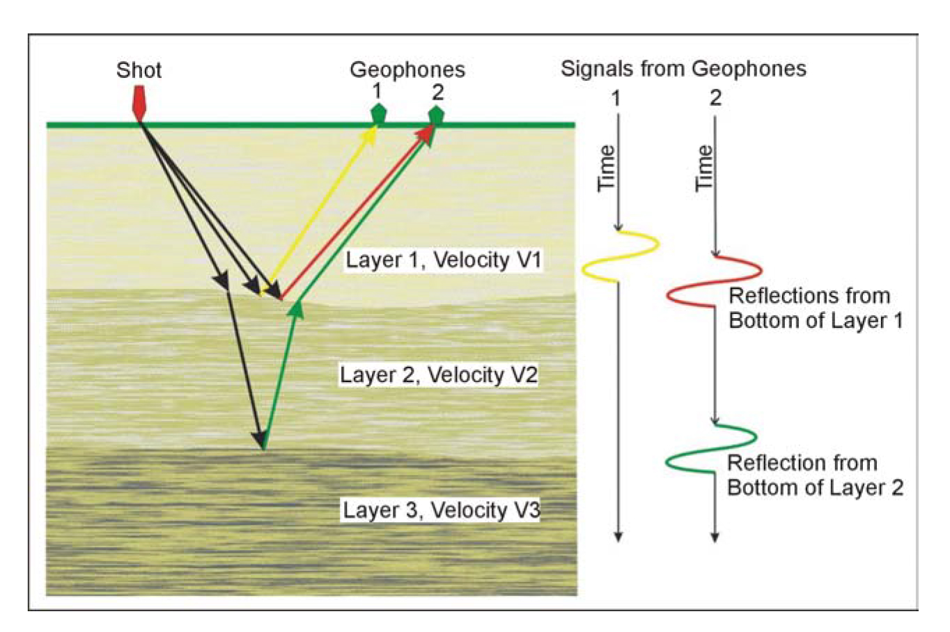
Figure 118. The SeismicReflection method.

Data Acquisition: A line of geophones is placed on the ground surface. Shots (hammer, drop weights or explosive sources) are initiated at regular intervals along the geophone spread and the resulting reflections are recorded by the geophones and stored in seismic recorder. Seismic reflection surveys require that the geophone and shot spacing are appropriate for the particular problem. The number of channels should be chosen so that the spread length is appropriate for the desired depth of investigation, and the geophone spacing needs to be such that the rugosity of the reflecting surface is imaged properly.

Data Processing: Many techniques are applied to process reflection seismic data. These include filtering, correcting for subsurface velocity effects, and stacking the traces that emanate from a common depth point (CDP) on the reflecting surface. The main objective of these techniques is to generate a gather (group) of seismic traces that can be stacked to image each reflection point as clearly as possible. The output from processing a line of seismic data is a seismic section showing the reflectors. This section can be presented as CDP location against record time, or when velocities are assigned to the different layers, as CDP against depth. More detail is provided in Part II Geophysical Methods, Theory and Discussion.

Data Interpretation: For reflection seismic surveys for bedrock depth determinations, a seismic section showing CDP against depth is most appropriate. Such a section should provide an immediate view of the depths to the bedrock.

Advantages: Seismic reflection generally requires a less intensive energy source for a given depth than the seismic refraction method. It is also better able to image greater depths than the refractions method.

Limitations: The seismic reflection method is usually fairly labor intensive and is often more expensive than other methods. In addition, when the bedrock depths are shallow, seismic refraction will usually be the more appropriate method. However, seismic reflection may be a more appropriate method when bedrock depths are more than 30 m.

Resistivity

Basic Concept: The resistivity method can be used to find bedrock depths if the overburden and bedrock have contrasting resistivities, which is usually the case. There are two common resistivity methods: soundings and traverses. Figure 119 shows the resistivity sounding method. Resistivity traverses are used to map lateral variations in resistivity and are not usually used to provide bedrock depths.

Data Acquisition: Figure 119a shows the system used to measure the resistivity of the ground. Current is passed into the ground using the two electrodes labeled A and B. The voltage that results from this current is then measured using electrodes M and N. Using the amount of current passed into the ground along with the voltage and a geometric factor for the electrode layout, the apparent resistivity of the ground is calculated. The electrode array is then expanded, making the current penetrate deeper into the ground and another reading is taken. This procedure is repeated for many electrode spacings, providing a set of apparent resistivity values for different electrode spacings. These values are plotted on a graph of resistivity against electrode spacing, as illustrated in Figure 119b. This graph shows that at small electrode spacings, the resistivity is that of the overburden. At large electrode spacings, the resistivity approaches that of the bedrock. The apparent resistivity curve is interpreted using software that provides a resistivity model (depths and resistivities) whose resistivity calculations match the field data.

Advantages: Unlike the seismic refraction method, which requires that each successive layer has a higher velocity, the resistivity method works whether the deeper layers become more or less resistive. The field procedures are fairly simple and a sounding to depths of about 50 meters depth can be conducted in less than one hour.

Limitations: Because electrodes need to be placed in the ground, the method is difficult to use in areas where the surface of the ground is hard, such as concrete or asphalt-covered areas. In addition, if the ground is dry, water may need to be poured on the electrodes in order to improve the electrical contact between the electrode and the ground. Generally, the separation between the current electrodes will need to reach a maximum of about three times the investigation depth. Thus, if the bedrock is 15 m deep, the current electrodes will need to be spaced up to 45 m apart. Lateral variations in resistivity can affect the accuracy of the depth interpretation, or grounded metal objects near the sounding site may also influence the data.

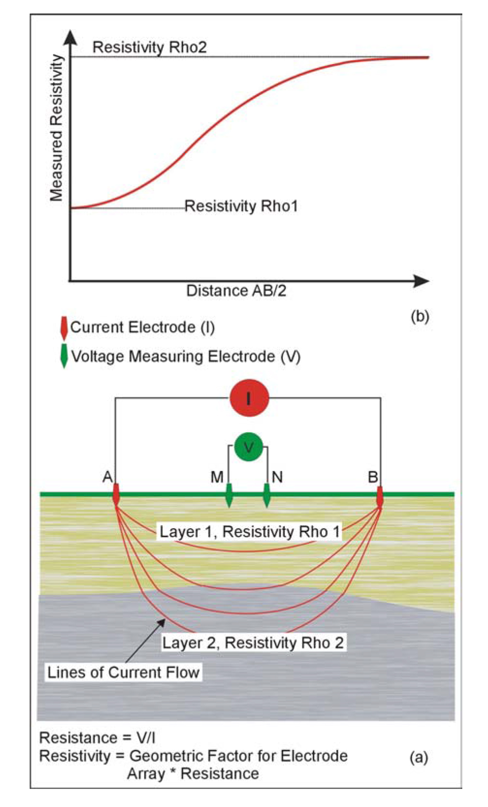
Figure 119. Resistivity Sounding (a) Data recording geometry, and (b) Sounding curve.

Time Domain Electromagnetic Soundings

Basic Concept: Time Domain Electromagnetic (TDEM) soundings are another method used to obtain the vertical distribution of the resistivity of the ground. This method is particularly well suited to mapping conductive layers, but can also be used to map resistive layers, which is likely to be the case for bedrock. To a significant degree, this method has now superseded the resistivity sounding method since it requires less work for a given investigation depth and generally provides more precise depth estimates. However, resistivity soundings are still useful for shallow investigations or when resistive targets are sought. Figure 120 provides a conceptual drawing of the TDEM method.

Data Acquisition: TDEM soundings are an electromagnetic method used to provide the vertical distribution of resistivity within the ground. A square loop of wire is laid on the ground surface. The side length of this loop is about half of the desired depth of investigation. A receiver coil is placed in the center of the transmitter loop. Electrical current is passed through the transmitter loop and then quickly turned off. This sudden change in the transmitter current causes secondary currents to be generated in the ground. The amplitude of these currents is related to the conductivity of each of the layers in the ground. Thus, the conductive layer will generate stronger secondary currents than a less conductive layer. The voltage measured by the receiver coil does not decay instantly to zero when the current is turned off but continues to decay for some time. This decaying voltage is caused by the decaying secondary electrical currents in the ground. The voltage measured by the receiver is then converted to resistivity.

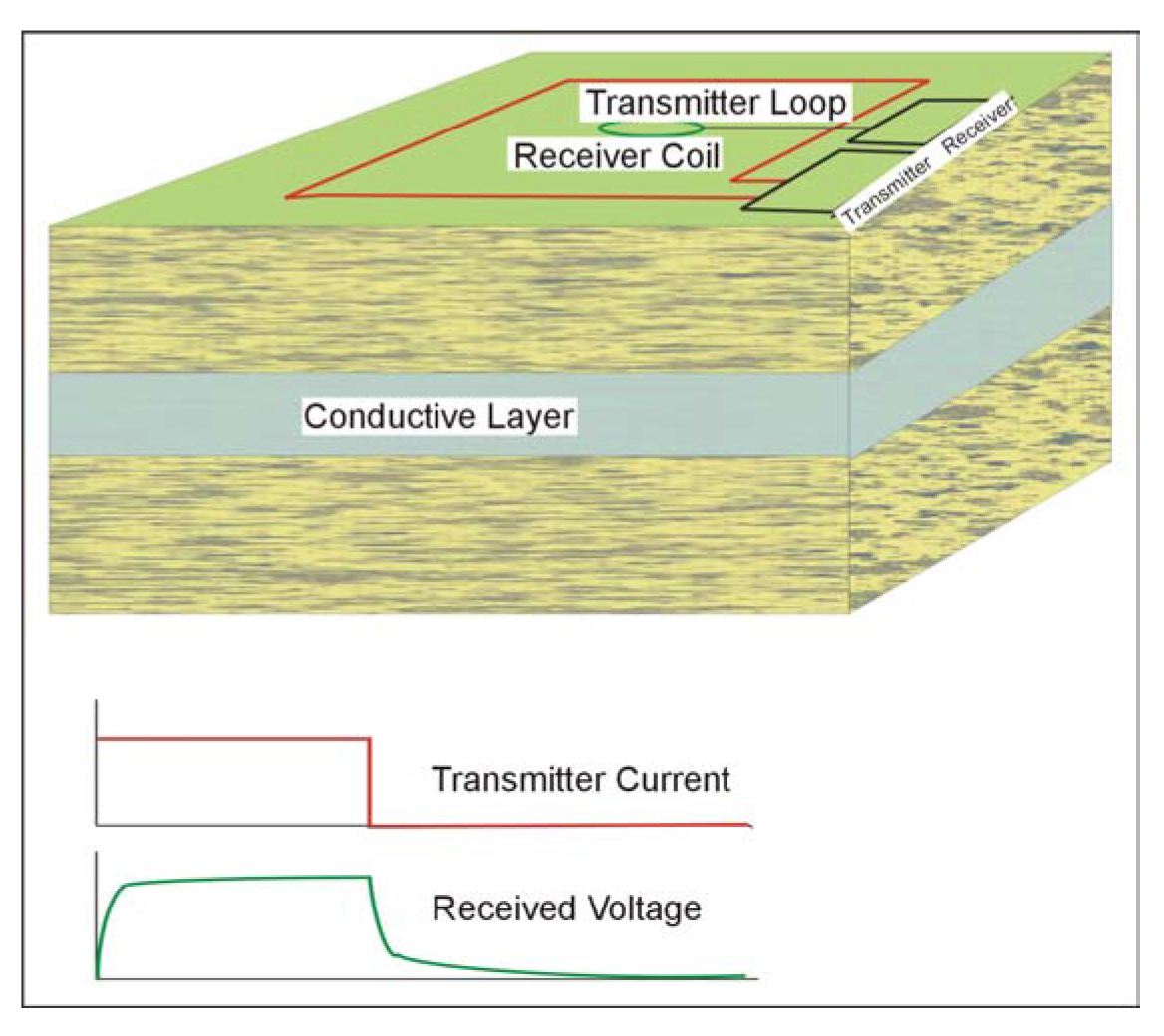
Figure 120. Time Domain Electromagnetic Soundings.

A plot is made of the measured resistivity against the decay time, as illustrated in Figure 121.

The switching and measuring procedure is repeated many times, which allows the resulting voltages to be stacked, thereby improving the signal-to-noise ratio. This procedure is repeated at different sounding locations until the area of interest has been covered. A sounding curve is plotted for each location showing the measured resistivity against decay time.

The resistivity sounding curve shown in Figure 121 illustrates the curve that would be obtained over three-layered ground. The near-surface layer is fairly resistive. This is followed by a layer having a much lower resistivity (higher conductivity) and causes the measured resistivity values to decrease. The third layer is again resistive.

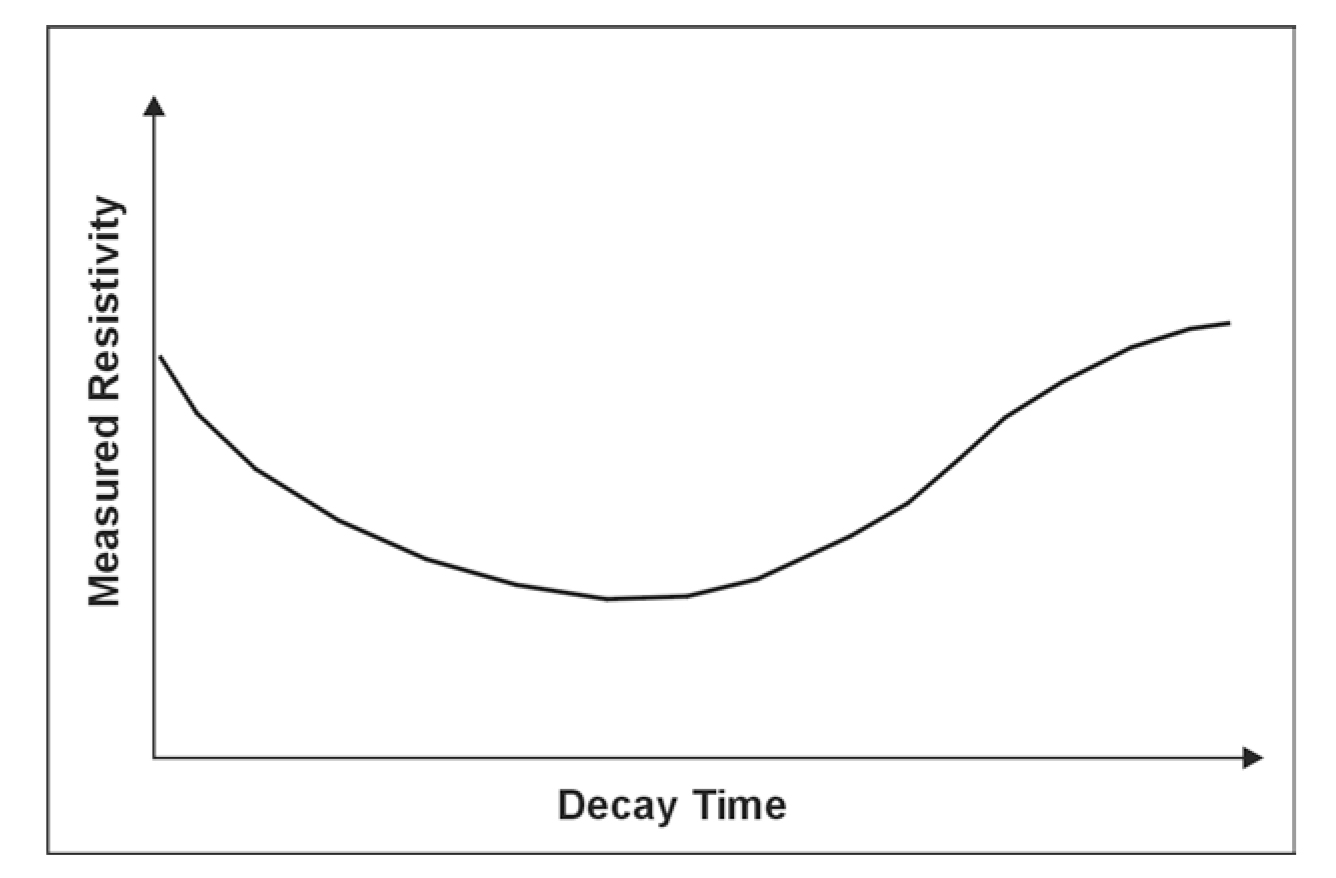
Figure 121. A Time Domain Electromagnetic Sounding curve.

Data Processing: The field data is transferred from the data recording instrument to a computer. The only processing required may be the removal of bad data. The data is then input to software that produces a sounding curve and facilitates interpretation.

Data Interpretation: The sounding curve is interpreted using computer software to provide a model showing the layer resistivities and thicknesses. The interpreter inputs a preliminary model into this software program, which then calculates the sounding curve for this model. It then adjusts the model and calculates a new sounding curve that better fits the field data. This process is repeated until a satisfactory fit is obtained between the model and the field data; this process is called inversion.

Advantages: Some of the advantages of the method have been mentioned under Basic Concept. The most important of these is that the method is often more efficient than the resistivity method, especially if the target is at depth greater than about 50 meters. In addition, compared to the resistivity method, the method is non-invasive and no electrodes have to be planted in the ground.

Limitations: TDEM soundings are an efficient method for investigating the vertical distribution of ground resistivity. Generally, the method is better suited to mapping conductive formations than resistive formations. However, it is also effective at mapping depths to resistive layers.

The most troublesome aspect of data recording is the influence of fences, power lines, and other "cultural" features. For surveys to determine the depth to bedrock near bridges and other structures, the metal in these structures may prohibit the use of this method. However, if the bedrock is fairly horizontal and soundings can be conducted some distance from the site, then TDEM surveys may still be appropriate.

Conductivity Measurements Using the EM31 and EM34

Basic Concept: If the bedrock has a significantly higher or lower conductivity than the overburden, its topography can be mapped using conductivity measurements. The concept is illustrated in Figure 122 where the bedrock has a higher conductivity than the overburden. When the conductive bedrock becomes deeper, then the measured conductivity decreases since it is more distant from the instrument. The reverse would occur if the bedrock had a lower conductivity than the overburden.

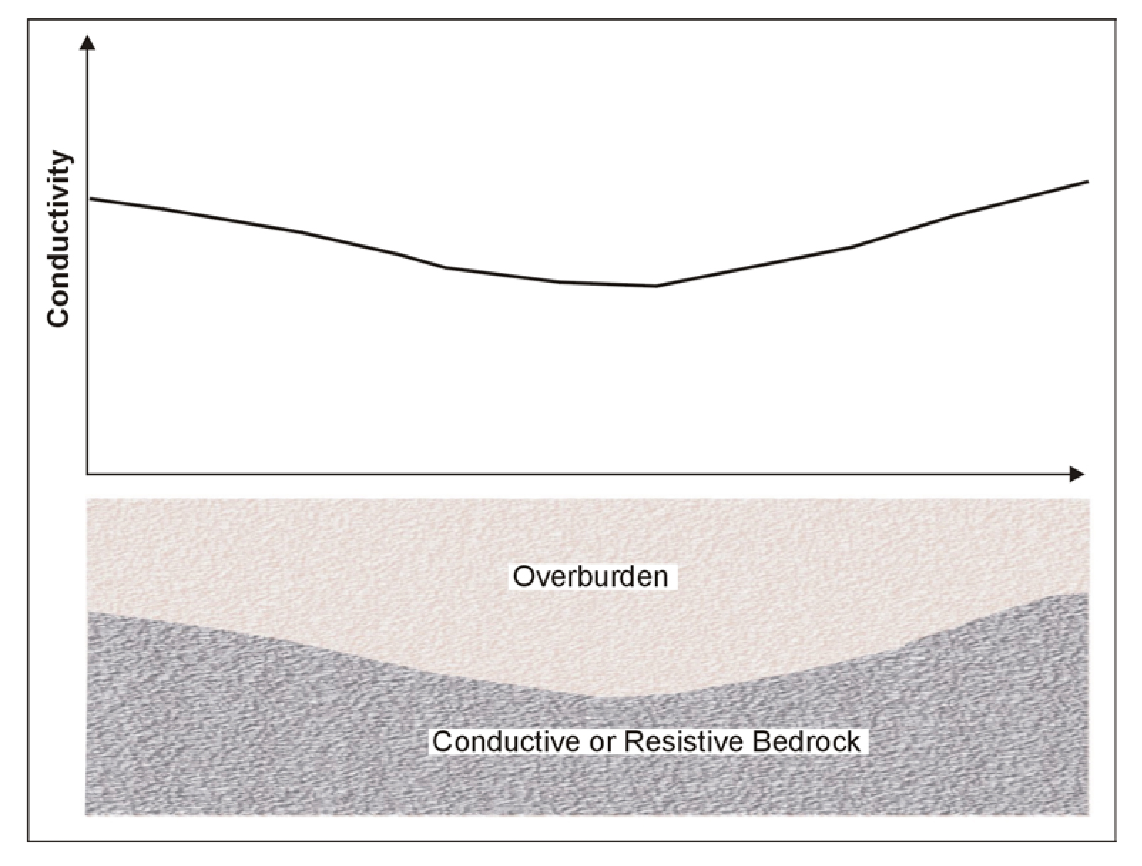
Figure 122. Model conductivity results over a conductive bedrock.

By mapping the conductivity of the ground to a depth sufficient to include the bedrock, the approximate topography of the bedrock can be ascertained. However, this method does not give the depth to the top of the bedrock. If this is required, resistivity soundings can be performed at selected points along the conductivity traverses. Using these data, the conductivity values can be converted to bedrock depths.

Data Acquisition: Conductivity surveys designed to map the topography of a conductive, or resistive, unit at depth (bedrock) will normally be conducted along lines crossing the area of interest. Several lines will be surveyed and conductivity data recorded. These lines will need to have their spatial coordinates surveyed to draw a map of the final data.

Probably the most important parameter that has to be determined before conducting the conductivity survey is the approximate depth of the bedrock and the configuration of the electromagnetic instrument to be used for the survey. The depth to the bedrock can be found from a resistivity sounding. This will also provide the electrical properties of the bedrock, indicating whether it is conductive or resistive compared to the overburden. The next step is to find the parameters of the electromagnetic measuring instrument required to image this bedrock surface. The EM31 and EM34 both have transmitters and receiver coils, which are coplanar. The transmitter produces sinusoidal electromagnetic waves oscillating at up to about 10 kHz, depending on the instrument, and, in the case of the EM34, the coil separation used. Measurements can be taken with the plane of these coils either parallel to the ground surface (vertical dipole mode) or normal to the ground surface (horizontal dipole mode). These two modes provide different depths of investigation and different responses to the geologic section. The vertical dipole mode provides greater depth of investigation. In this mode, the conductivity readings are less sensitive to near-surface changes in conductivity. In the horizontal dipole mode, the depth of investigation is less than the vertical dipole mode, and the measured conductivity values are more sensitive to near-surface changes in conductivity.

The transmitter and receiver coils are mounted in a rigid boom in the EM31 and are, therefore, fixed (Figure 183).

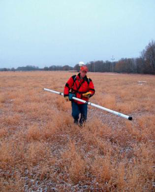
Figure 183. The EM31 MK2 instrument. (Geonics, Ltd.)

With the EM34, the coils are not mounted in a rigid structure, and the distance between them can be changed to provide increasing depths of investigation with increasing separation between the coils. Figure 197 shows the EM34 being used in the horizontal dipole mode.

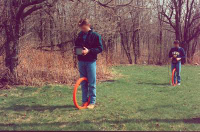
Figure 197. The EM34 is being used in horizontal dipole mode. (Geonics, Ltd.)

In order to check whether the conductivity measurements are responding to a depth sufficient to image the bedrock, measurements can be taken with the EM34 using the two modes at each of the three coil spacings allowed. Since the contrast between the overburden and bedrock are known from the resistivity sounding, the EM34 measurement parameters needed to image the bedrock can be found. This then sets the EM34 data recording parameters to be used for the survey.

Data Processing: Usually little processing is done to the data although it may sometimes be necessary to remove bad data points.

Data Interpretation: Interpretation is often visual, looking for the conductivity lows for deeper sections of the conductor, or conductivity highs if the bedrock is more resistive than the overburden. If resistivity soundings have been recorded, the conductivity values can be converted to depth, as described earlier.

Advantages: The prime advantage of the method is that it can provide a rapid method of mapping approximate bedrock topography.

Limitations: The bedrock layer has to be thick enough to have a significant influence on the conductivity readings. In addition, it has to be more conductive, or resistive, than the overburden. If shallower conductive layers occur, or possibly fade in and out spatially, this may obscure the interpretation of the deeper conductive layer. Any metal, either above or below the ground surface local to the instrument will negatively influence the data.

Spectral Analysis of Surface Waves

Basic Concept: The Spectral Analysis of Surface Waves (SASW) method is used to measure the layer depth and shear wave velocity of the ground. Rather than responding to discrete layers, this method provides a more general (bulk) shear wave velocity along with the depth at which this velocity changes. The method may be used for investigating bedrock properties for foundation studies.

The method is based on the propagation of mechanically induced Rayleigh waves. By striking the ground surface with a hammer or other source, a transient stress wave is created, including surface or Rayleigh waves, which are registered by two transducers placed in line with the impact point on the ground surface at fixed separations. The transducers, which may be small accelerometers, register the passage of the waves. The receiver outputs are plots of the phase difference between the two transducers as a function of frequency. A profile of Rayleigh wave velocity versus wavelength, or so-called dispersion curve, is calculated from the phase plot. The ratio of Rayleigh wave velocity to shear wave velocity is approximately 0.9:1; thus, the shear wave velocity can be estimated. The shear stiffness (G) of the ground can be calculated from the shear velocity if the material density is known and a plot of ground stiffness as a function of depth from the surface can be obtained.

Rayleigh waves have velocities that depend on their wavelength, a phenomenon called dispersion. Waves having different wavelengths sample to different depths, with the longer wavelengths sampling to greater depths. Figure 35 illustrates the sampling depths and particle motion of two Rayleigh waves having different wavelengths.

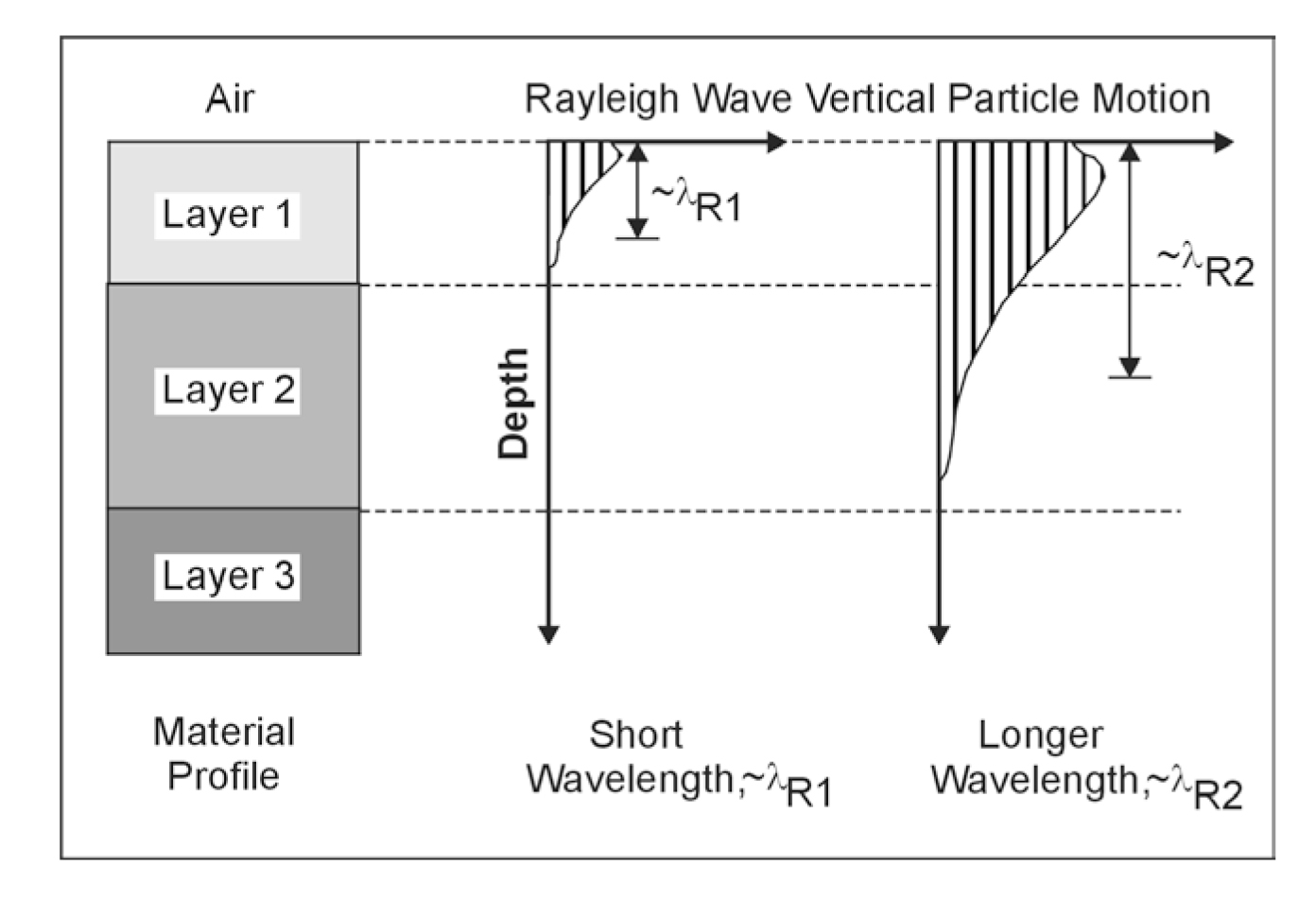
Figure 35. Schematic showing variation of Rayleigh wave particle motion with depth.

This principle is used to measure the thickness of ground layers with different stiffness properties. It can also be used to locate and roughly delineate inhomogeneities such as voids.

Data Acquisition: The SASW field setup is shown in Figure 36. Either a transient or continuous point source is used to generate Rayleigh waves, which are monitored by two in-line receivers. The data acquisition system calculates the phase difference between the receiver signals. These phase data are processed later into the dispersion curve, which is modeled analytically to determine a compatible shear wave velocity profile for the site. The data acquisition system is discussed in more detail below.

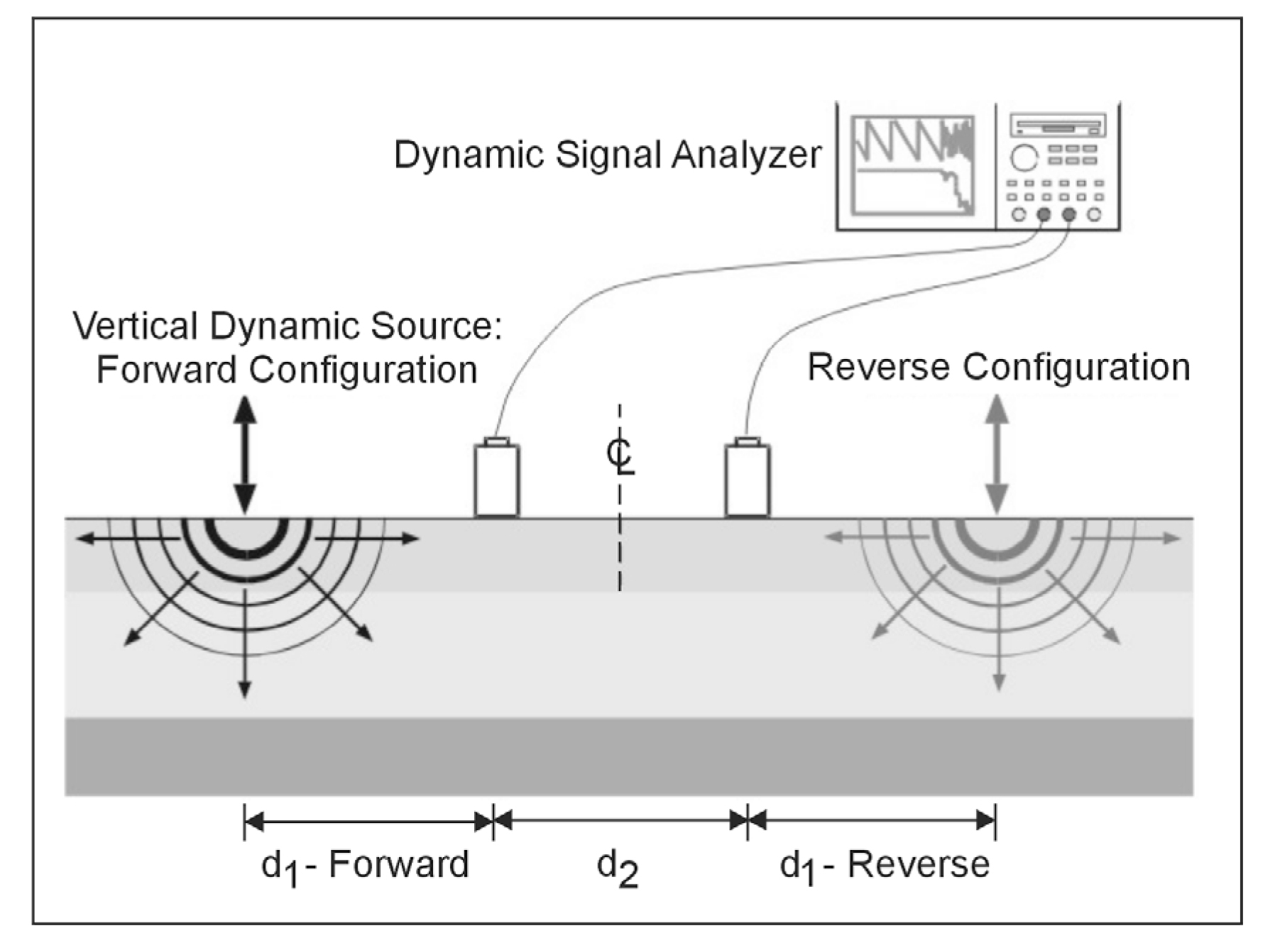
Figure 36. Basic configuration of Spectral Analysis Surface Waves measurements.

The source used depends on the desired profiling depth. Heavier sources generating lower frequency waves provide deeper interpretations. A combination of sources is commonly used to measure dispersion over a broad enough bandwidth to resolve both the near-surface and greater depth. Transient sources include sledgehammers (<15 m depth) and dropped weights. Continuous sources include the electromagnetic vibrator (<40 m depth), eccentric mass oscillator, heavy equipment such as a bulldozer (30 to 150 m depth), and the vibroseis truck (<120 m depth). A pair of vertical receivers monitors the seismic waves at the ground surface. For profile depths of around 100 m, 1-Hz geophones are required. Five or 10-Hz geophones can be used for surveys from 10 to 30 m deep. Theoretical as well as practical considerations, such as attenuation, necessitate the use of an expanding receiver spread. Data are recorded from sources placed on both sides of the geophones, providing both the forward and reverse direction shots (Figure 36).

Data Processing: In the SASW method, a Fast Fourier Transform (FFT) analyzer or PC-based equivalent is used to calculate the phase data from the input time-voltage signals. Typically, only the cross power spectrum and coherence are recorded. Coherent signal averaging is used to improve the signal-to-noise ratio, a process similar to stacking. Because of the initial processing done by the analyzer in the field, the effectiveness of the survey can be assessed and modified if necessary. An initial estimate of the shear wave velocity (V_S) profile can be made quickly.

Data Interpretation: Interpretation consists of modeling the surface wave dispersion to determine a layered V_S profile that is compatible. Interpretation can be done on a personal computer.

The acquisition and processing techniques of SASW methods do not separate motions from body wave, fundamental mode Rayleigh waves, and higher modes of Rayleigh waves. Usually, it is assumed that fundamental mode Rayleigh wave energy is dominant, and forward modeling is used to build a 1-D shear wave velocity (V_S) profile whose fundamental mode dispersion curve is a good fit to the data.

The major advantages of the SASW method are that it is non-invasive and non-destructive, and that a larger volume of the subsurface can be sampled than in borehole methods.

Limitations: The depth of penetration is determined by the longest wavelengths in the data. In modeling, there is a trade-off between resolution (layer thickness) and variance (change in V_S between layers). Data that is noisier must be smoothed and will have less resolution because of this. Whether a particular layer can be resolved depends on its depth and velocity contrast. The modeled shear wave velocity (V_S) profile is not sensitive to reasonable variations in density. The compressional wave velocity (V_P) cannot be resolved from dispersion data, but has an effect on modeled V_S. The difference in V_P in saturated versus unsaturated sediments causes differences of 10% to 20% in surface wave phase velocities, which leads to differences in modeled V_S.

The depth of penetration is determined by the longest wavelengths that can be generated by the source, measured accurately in the field, and resolved in the modeling. Generally, heavier sources generate longer wavelengths, but site conditions are often the limiting factor. The available open space determines the offset from the source and aperture of the array, which determines the near-field wave filter criteria. Commonly, wavelengths are removed from the data that are longer than twice the distance between the receivers. Attenuation characteristics of the ground determine the signal level at the geophones. The cultural noise (traffic, rotating machinery) at a site may limit the signal-to-noise ratio at low frequencies. In SASW methods, the depth of resolution is usually one-half to one-third of the longest wavelength. Surveys to depths of 100 m are reported using heavy equipment for the seismic source. With a hammer source, depths up to about 20 m may be expected. Exploration depths of 1 m, or maybe less, are possible.

The field setup requires a distance between the source and most distant geophone of two to three times the resolution depth. However, forward modeling allows for subjective interpretation of the sensitivity of the dispersion curve to the layered V_S model. Resolution decreases with depth. A rule of thumb is that if a layer is to be resolved, then the layer thickness (resolution) should be at least around one-fifth of the layer depth.

The SASW method is applicable for measuring the bulk shear and compressional wave velocities of the soil and overburden. It is used in earthquake-prone areas to evaluate the engineering properties of the soil/overburden to depths of about 30 m.

Multi-Channel Analysis of Surface Waves

The most common surface wave method today for geotechnical investigations is multi-channel analysis of surface waves (MASW). MASW typically uses a linear, L-shaped, or circular array of geophones (typically 24 or 48) for measuring the surface wave dispersion curve. The dispersion curve is then inverted to determine the corresponding shear wave velocity profile. MASW data can be acquired with an active sound source similar to SASW, or using ambient noise. The method provides Vs information in either 1D (depth) or 2D (depth and surface distance) formats.

Basic Concept: Using an array of geophones connected to a multi-channel seismograph, seismic travel-times, amplitudes, and frequency of energy created by hammer blows to the ground surface is measured. As an alternative method, ambient seismic noise can also be recorded. Such noise, sometimes called microtremors, is constantly being produced by cultural and natural noise.

Because MASW processing schemes utilize a wavefield transform applied to the field data, the method has the capability to automatically account for adverse affects of near-field, far-field, spatial aliasing, and ambient energy. Therefore, acquisition parameters for MASW have a wide range of tolerance, unlike conventional refraction and reflection seismic surveys. The two most important parameters to be considered for MASW surveys are the source offset and the receiver spacing. These parameters are dependent on the site conditions and the average stiffness of the near-surface geologic materials.

The MASW method can be used to determine shear wave profiles to depths of up to 30 meters. However, due to the dispersive nature of surface waves with longer wavelengths penetrating deeper into the subsurface than shorter wavelengths, resolution decreases significantly with depth.

Data Acquisition: For a 2D investigation, the seismic equipment is laid out in an array very similar to that used in seismic refraction surveys. A multiple number of receivers (usually 24 or more) are deployed with an even spacing along a linear survey line with geophones connected to a multi-channel seismograph. Each channel is dedicated to recording vibrations from one receiver. Typically records of 1 second are stored in the seismograph from impacts to the surface repeated several times for signal stacking, using a 1 millisecond sample interval. One multichannel record, commonly referred to as a shot gather, consists of a multiple number of time series (called traces) from all the receivers in ordered manner (i.e., 1 through 24). When recording ambient noise, record time is typically 10-15 minutes.

Since the equipment and setup is very similar to the one used for seismic refraction, it can often be beneficial to collect refraction and MASW data simultaneously.

Data Processing and Interpretation: The data is processed using one of several commercially available software packages. MASW interpretation requires no prior assumptions about the subsurface structure. Data processing is a complex series of iterative sequences combining shot gathers, analyzing each shot record for dispersion of the surface waves recorded, inverting the dispersion curve to 1D Vs profiles, and combining the 1D profiles into 2D cross sections. Figure 123 illustrates the process flow for analysis and interpretation of MASW data.

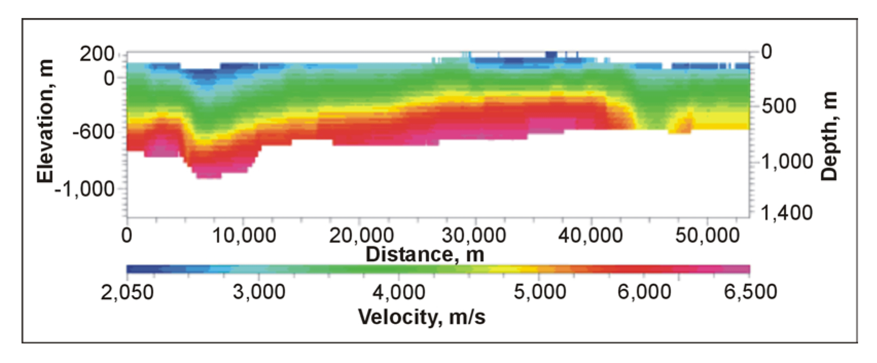
Figure 123. Illustration of the process used to derive MASW shear wave velocity (2D) cross-sections (from Kansas Geologic Survey).

If a 1D shear wave velocity profile is required, then 1D MASW method can be used. Figure 124 shows a shear wave profile with the ReMi results being compared with a shear wave velocity log. Such results may be useful for several applications including soil compaction control, pavement evaluation, mapping the subsurface and estimating the strength of subsurface materials and finding buried cultural features such as dumps and piers.

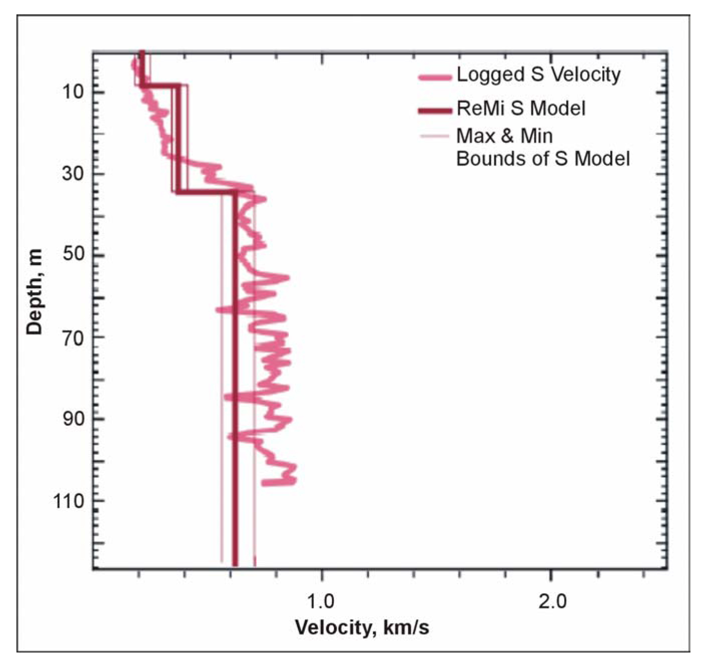
Figure 124. Shear-wave profile interpretation from a SeisOpt survey.

Advantages: The method is reported to have a wide range of applications, including rippability studies, void and utility detection, basement mapping and fault mapping. In addition, the 1D MASW method, which with the right setup can determine shear wave velocities to depths of 30 meters, can be used to determine the NEHRP soil classification at a site.

Limitations: Since the method is relatively new, the limitations may not yet be apparent. However, since the method partly relies on ambient noise, it is possible that all of the frequencies required for a particular target may not be present at a particular site. At some sites, such as near a busy highway, the frequencies may be dominated by a small range of frequencies having a high amplitude. Resolution decreases quickly with depth which limits the ability to detect thinner layers at depth.

Gravity

Basic Concept: The gravity method measures small spatial differences in the gravitational pull of the Earth. If the bedrock and overburden have different densities, the gravity pull will change over bedrock topographic features.

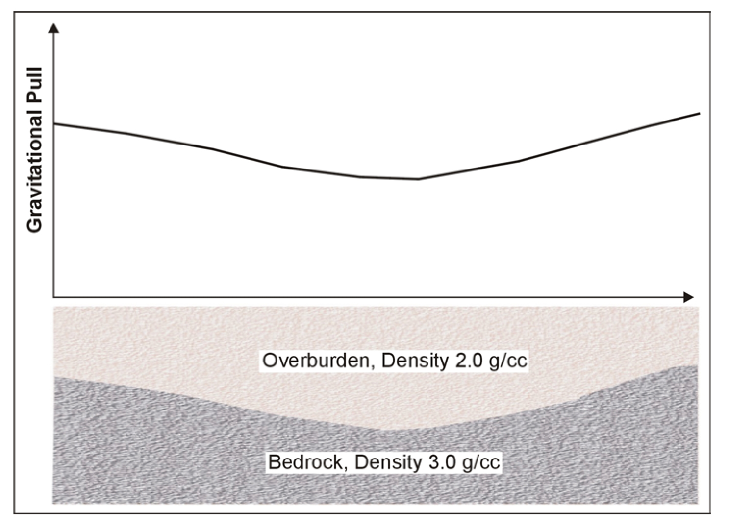
Figure 125. Gravitational pull over a bedrock depression.

In Figure 125, the bedrock is assumed to have a density of 3.0 g/cc, and the overburden has a density of 2.0 g/cc. Since the bedrock density is greater than that of the overburden, the gravitational pull at the ground surface is higher when the bedrock is nearer the ground surface.

The instrument used to measure the gravity pull is called a Gravimeter. This instrument does not record the absolute value of the pull of gravity but measures spatial differences in the gravity pull.

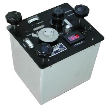
Figure 126. Lacoste and Rhomberg model D1a gravity meter. (LaCoste & Romberg)

The anomalous gravitational field over a bedrock structure (depression or mound) depends on the amplitude of the depression, its width and depth, and the density contrast between the overburden and the bedrock. Significant bedrock topography with large density contrasts will produce large gravitational anomalies. Conversely, small amplitude structures at depth, even with large density contrasts, may produce only very small anomalies. Clearly, the size of an anomaly depends on the parameters of the structure and its depth, and, at some point, it cannot be observed. Thus, it is important to be able to measure the gravity field with as much accuracy as possible. The Lacoste and Rhomberg model D meter has an advertised accuracy of 10 microgals (980,000,000 microgals is the Earth's gravitational field). Variations in gravity anomalies found over topographic changes in bedrock vary from undetectable to hundreds of microgals. Figure 126 shows the Lacoste and Rhomberg model D1A gravity meter.

This is one of the preferred instruments for measuring small changes in the gravitational pull. If only very small anomalies are expected, the Lacoste and Rhomberg model EG can be used (Figure 85). This instrument has an advertised repeatability of 3 microgals.

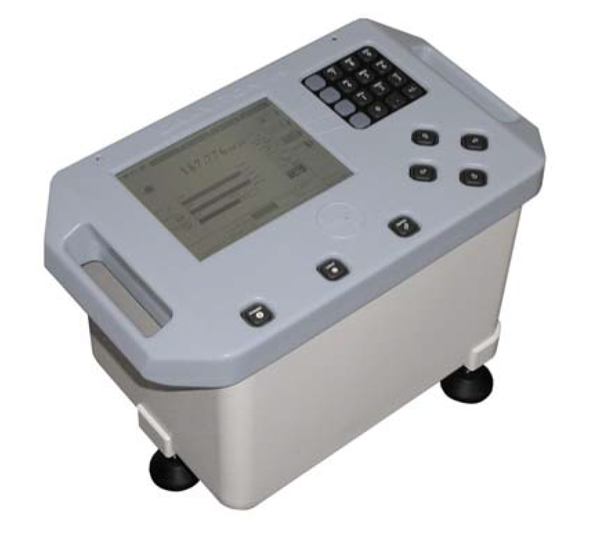
Figure 85. Gravity EG gravity meter. (LaCoste & Romberg)

Data Acquisition: Surveys are usually conducted along lines crossing the area of interest. The expected size of the bedrock feature will determine the distance between readings (station spacing). A spatially small bedrock feature will require a smaller station spacing than that which would be required for a large bedrock feature. It is usually advisable to model the expected anomaly mathematically before conducting fieldwork. From this, along with the expected instrument accuracy, an estimate can be made of the anomaly size and the required station spacing.

Surveys are conducted by taking gravity readings at regular intervals along a traverse that crosses the expected location of the bedrock topography. However, in order to take into account the expected drift of the instrument, one station (probably the first) has to be reoccupied every half hour or so (depending on the instrument drift characteristics) in order to obtain a field graph of the instrument drift. Since gravity decreases with distance from the center of the earth, the elevation of each station has to be measured to an accuracy of about 3 cm.

Data Processing: Several corrections have to be applied to the field gravity readings. Each reading has to be corrected for elevation, the influence of tides, latitude, and, if significant local topography exists, a topographic correction. In a modern instrument such as the Lacoste and Rhomberg model D, the meter may do tidal and drift corrections.

Data Interpretation: Gravity data are interpreted using software to calculate the gravity field of geologic features input by the operator. The program will then change the parameters (shape, depth) of the body (in this case, bedrock topography) until the calculated gravity field matches the observed gravity field. This process is called inversion and is commonly used in geophysical interpretation. If several lines of data have been acquired, a map of the gravity field may be produced.

Advantages: Gravity surveys require only a small amount of instrumentation (a gravity meter and instrument for elevation control). Gravity surveys are unobtrusive and can be conducted in environmentally sensitive areas.

Limitations: Gravity surveying is a labor-intensive procedure requiring significant care by the instrument observer. These instruments require careful leveling, although some of them are self-leveling, such as the Lacoste and Rhomberg EG. Once the reading has been taken, the gravity sensing mechanism must be clamped to stop excessive vibration, which would alter the readings. The instrument must be placed on solid ground (or a specially designed plate) so that it does not move (sink into the ground) while the reading is being taken. As mentioned above, all of the stations have to be surveyed for elevation.

The anomaly from bedrock topography rapidly becomes smaller with depth, and, therefore, detectability rapidly decreases with depth. Pre-survey modeling is important to establish the expected anomaly size and to determine if a gravity survey is feasible.

If other layers are present between the surface and bedrock, and these layers vary laterally in thickness or density, they will create gravity anomalies that may hinder an interpretation of the bedrock topography. In addition, fracture zones and voids may also create anomalies that may hinder an interpretation of bedrock depth.

Methods to Map Fractures

As with any geophysical method, fractures must present some physical property or contrast that can be detected from the ground surface. Generally, geophysical methods will not detect individual fractures unless they are large, but can detect fracture zones. Usually, fractures in the bedrock will contain more moisture than the host unfractured rock, and, therefore, will be more electrically conductive. They will also probably be areas of lower seismic velocity than unfractured bedrock. In some cases, since fractured areas are more subject to erosion, the fractured region may represent as a topographic depression with the surrounding unfractured bedrock higher. Figure 127 presents a pictorial view of a fracture and the potentially useful attributes.

Several geophysical methods can be used to map bedrock fractures. The most commonly used methods are listed below:

1. Conductivity Measurements
2. Ground Penetrating Radar
3. Rayleigh waves recorded with a Common Offset Array (Common Offset Surface Waves)
4. Seismic Refraction
5. Shear Wave Seismic Reflection
6. Resistivity Measurements

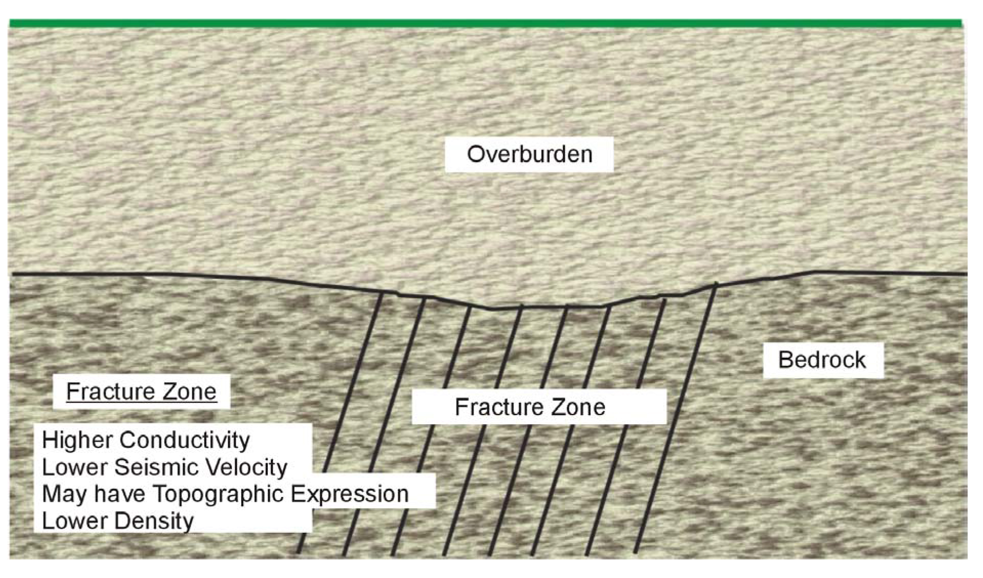
Figure 127. Bedrock fractures and potentially useful attributes.

The theory of all of these methods except Common Offset Surface Waves and Shear Wave Seismic Reflection has been described earlier and will not be presented in this section. However, there are some differences in the application of the above listed methods for locating fractures, which will be discussed where appropriate. The theory of Common Offset Surface Waves and Shear Wave Seismic Reflection will be briefly described

Conductivity Measurements to Map Fractures

Basic Concept: Conductivity measurements can be made with either the EM31 or EM34 in vertical dipole mode to locate conductive fracture zones. The anomaly measured in the vertical dipole mode is quite distinctive and is diagnostic of a vertical, or sub vertical, conductive feature. Figure 128 shows the anomaly over a conductive feature using an EM31 or EM34 in vertical dipole mode.

The measured conductivity increases as the conductive feature is approached. When the transmitter and receiver coils straddle the conductive zone the measured conductivity values decrease, reaching a minimum when they are equispaced about the conductive zone. This distinctive anomaly shape provides a good method for locating conductive fractures.

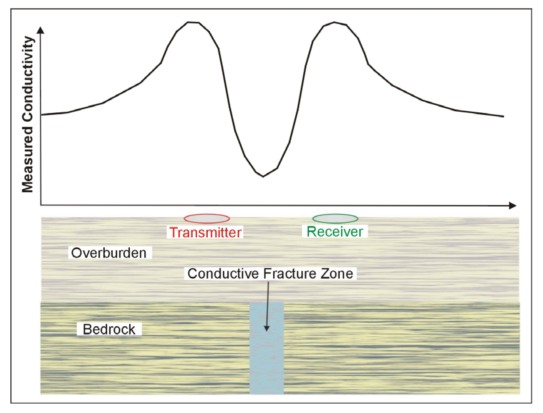
Figure 128. Anomaly from an EM31/34 used in vertical dipole mode over a conductive fracture zone.

Ground Penetrating Radar to Map Fractures

Ground Penetrating Radar (GPR) can be used to locate fractures and fracture zones. Reflections obtained over a fracture zone are more likely to be scattered than those emanating from the bedrock. This may allow fractured areas to be recognized. Figure 129 shows a GPR section over a fracture zone. In this case, the fracture is sub-horizontal and is seen as a reflector on the GPR section. Basic Concept, Data Acquisition, Data Processing, Data Interpretation, Advantages and Limitations were discussed in a previous section.

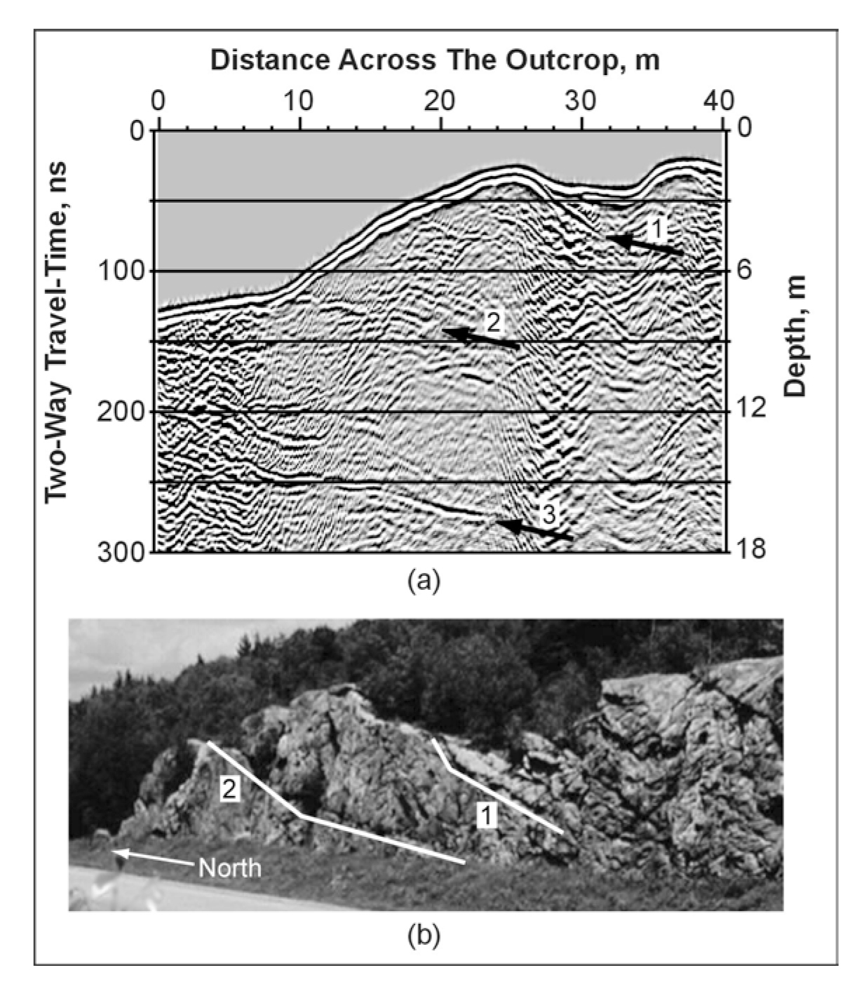
Figure 129. Ground Penetrating Radar data illustrating a section over a fracture zone. (Lane, 2000).

Rayleigh Waves Recorded with a Common Offset Array to Map Fractures

Basic Concept: This method uses Rayleigh waves (surface waves) to detect fracture zones. Rayleigh waves have a particle motion that is counterclockwise with respect to the direction of travel. Figure 130 illustrates the particle motion for Rayleigh waves traveling in the positive X direction. In addition, the particle displacement is greatest at the ground surface, near the Rayleigh wave source, and decreases with depth. Three shot points are shown, labeled A, B, and C. The particle motion and displacement are shown for five depths under each shot point. For shot B over the fracture zone, the amplitude of the Rayleigh waves is smaller than that for the other shots due to attenuation caused by the fractures. This affects the measured Rayleigh wave recorded by the geophones over the fracture zone. The effective depth of penetration is approximately one-third to one-half of the wavelength of the Rayleigh wave.

For interpretation, three parameters are usually observed. The first is an increase in the travel time of the Rayleigh wave as the fracture zone. The second parameter is a decrease in the amplitude of the Rayleigh wave. The third parameter is reverberations (sometimes called ringing) as the fracture zone is crossed. The data are recorded using a seismograph and geophone.

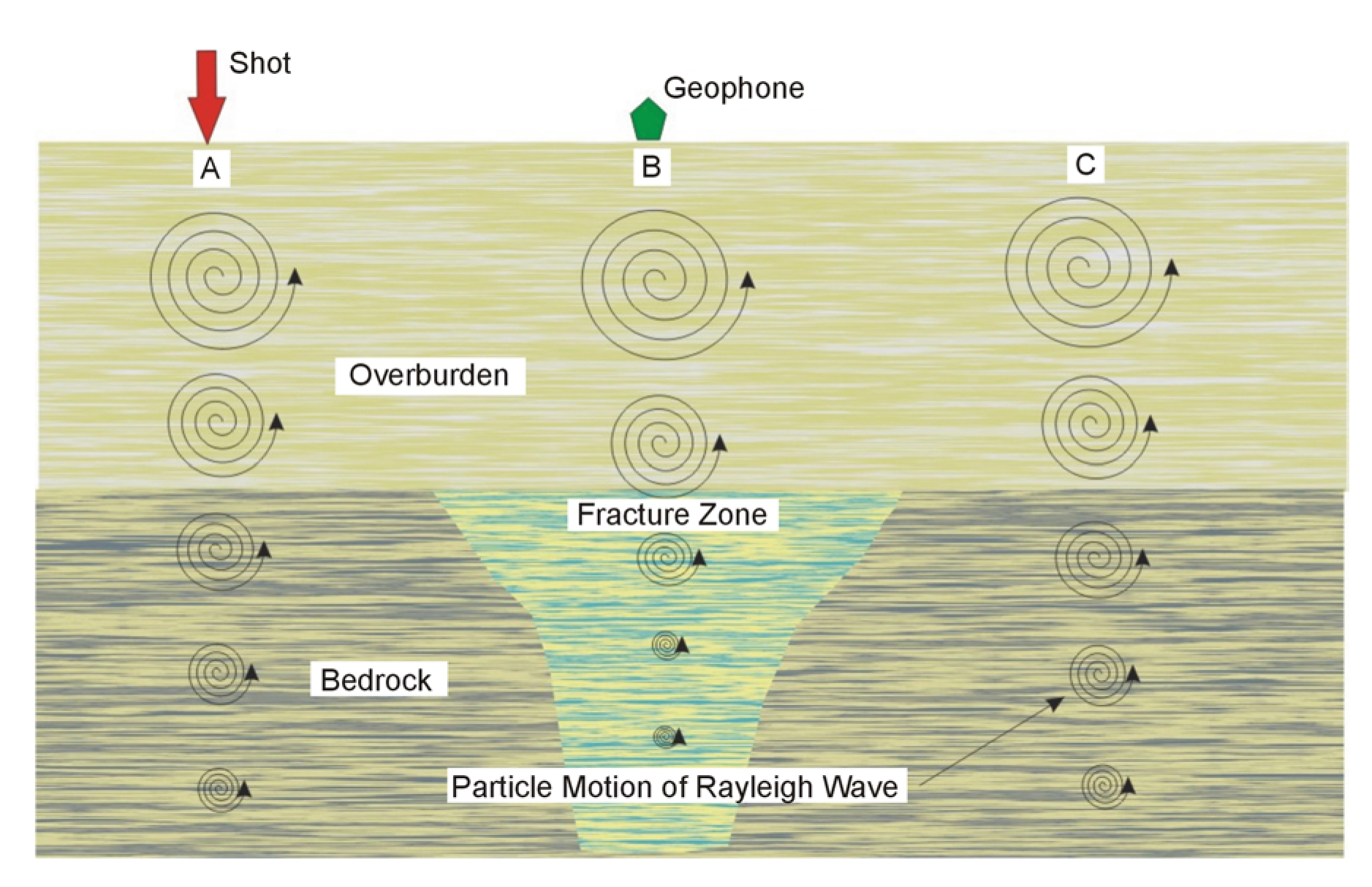
Figure 130. Rayleigh wave particle motion and displacement over a fracture zone.

Data Acquisition: Rayleigh waves are created by any impact source. For shallow investigations, a hammer is all that is needed. Data is recorded using one geophone and one shot point. The distance between the shot and geophone depends on the depth of investigation and is usually about twice the expected target depth. Data are recorded at regular intervals across the traverse while maintaining the same shot geophone separation. The interval between stations depends on the expected size of the fracture zone and the desired resolution. Generally, to clearly see the fracture zone, it is desirable to have at least several stations that cross this area. Figure 100 presents data from a common offset Rayleigh wave survey over a void/fracture zone in an alluvial basin. The geophone traces are drawn horizontally with the vertical axis being distance (shot stations).

Data Processing: The data may be filtered to highlight the Rayleigh wave frequencies and is then plotted as shown on Figure 100. Spectral analysis can be performed on the individual traces and may show the lower frequencies over the fracture zone.

Figure 100. Data from Rayleigh wave survey over a void/fracture zone.

Data Interpretation: The data shown in Figure 100 illustrates many of the features expected over a void/fracture. The travel time to the first arrival of the Rayleigh wave is greater across the void/fracture and is wider than the actual fractured zone. The amplitudes of the Rayleigh waves decrease as the zone is crossed. Since the records are not long enough, the ringing effect is not presented in these data.

Advantages: The field data recording is simple and efficient and requires much less effort for a given line length than seismic refraction.

Limitations: The method responds to the bulk seismic properties of the rocks and soil, which are influenced by factors other than voids. It has a limited depth of penetration and resolution. Penetration depth is limited by the wavelengths generated by the seismic source. However, this method is faster and less costly than most other seismic methods.

Seismic Refraction to Map Fractures

Basic Concept: The seismic refraction method can be used to locate fracture zones. Surveys for fracture zones are somewhat different from the more conventional application of the seismic refraction method described earlier, which is mapping bedrock topography. Bedrock fracture zones are recognized from the character of the first signal arrivals at the geophones, which can attenuate the signal and cause time shifts, as is illustrated in Figure 131.

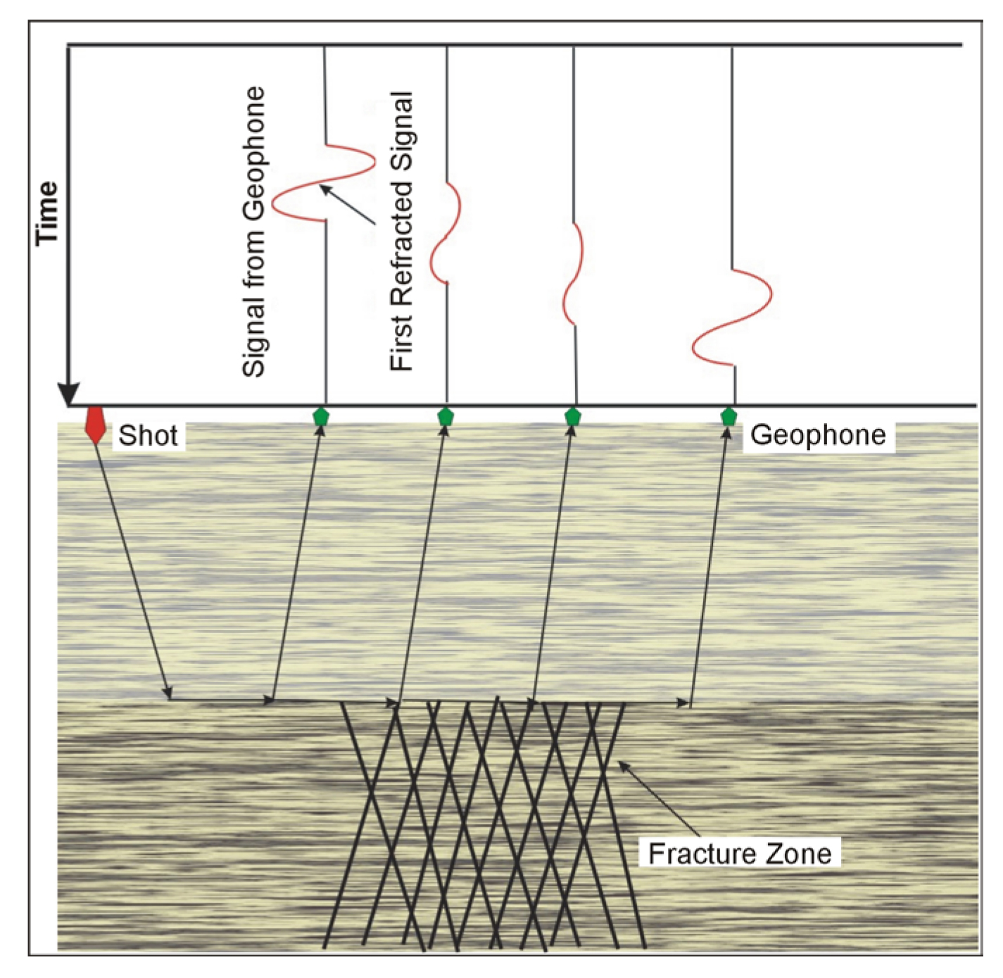
Figure 131. Seismic Refraction for locating fracture zones.

In addition to compressional wave surveys for fracture zones, shear waves can also be used. If a shear wave is oscillating at right angles to its direction of travel, it will be severely attenuated over a fracture zone. If, however, the shear wave is oscillating along the direction of travel, it will be relatively unaffected by the fracture zone.

For compressional wave surveys, surveys are conducted by traversing across the area of interest and evaluating the character of the first arrival waveform.

Data Acquisition: Data is recorded by placing a line of geophones across the area of interest and recording data from shots placed at the ends of the geophone spread.

Data Processing: No processing is usually required. The data is plotted so as to allow the character and amplitude of the first waves to arrive to be viewed.

Data Interpretation: The data is interpreted by viewing the first wave arrivals and looking for waves whose amplitude is diminished, indicating that a fracture zone has been crossed.

Advantages: Field recording for this method is quite fast and the data can usually be viewed on the recorder screen as the survey progresses.

Limitations: The velocity of the bedrock has to be greater than that of the overburden. If the water table is near the bedrock then this may also provide refractions. These refractions may interfere with refractions from the bedrock, or the bedrock refractions may not be visible.

Shear Wave Seismic Reflection to Map Fractures

Basic Concept: Fracture zones can be detected using seismic shear wave reflection surveys. These surveys are conducted in much the same manner as compressional wave seismic reflection surveys, except that a shear wave source and geophones have to be used. Near-surface shear-wave seismic surveys typically employ horizontally polarized (SH) waves because they are more easily distinguished from compressional (P) waves, and they generally do not convert to P waves as readily as vertically polarized shear (SV) waves. SH waves are generated by inputting horizontal ground motion at the earth's surface by striking a fixed object with good coupling to the ground from the side. This is accomplished using some combination of mass holding the object down and spikes holding it laterally stable. There are also SH sources (one called the Microvib and is shown in Figure 95). The data are recorded using a standard seismograph (Figure 114b) using shear wave geophones.

Figure 95. The Microvib shear wave generator. (Bay Geophysical)

Figure 114. Seismic Refraction: field set up and data recorder.

Data Acquisition: Probably the most important difference between shear wave and compressional wave surveys is that, for shear wave surveys, the geophone spacing will be smaller for an equivalent depth of investigation, since the velocity of shear waves is only about 0.6 times that of compressional waves. The geophone spacing and spread length are also dependent on the expected depth and size of the fracture zone. Another important quantity to consider is the frequency and wavelength of the shear waves. Higher frequencies provide better resolution of the detected structures. However, higher frequencies also attenuate faster and therefore have less depth penetration.

Data Processing: Data processing is essentially the same as for reflection seismic surveys. Since the data are recorded in shot mode, the records are sorted to gathers with a common midpoint. Various kinds of filtering and other processes are then used to refine the data after which the traces for each gather are summed to produce a single trace whose signal-to-noise ratio is much greater than the unprocessed traces. Once this procedure has been done for all traces, a plot can be produced showing the seismic reflectors. Additional processing, such as migration, can also be applied to these data.

Data Interpretation: Data interpretation consists mostly of visual observation of the processed seismic records. Fracture zones produce scattering of the seismic energy, resulting in less energy being reflected back to the geophones on the ground surface. Areas where the amplitude of the bedrock reflector decreases or fades out will be of interest. In addition, an increase in travel time to the bedrock reflector may also occur. Figure 98 shows a shear wave seismic section, although in this case the target was voids. However, it does illustrate the presentation of the data.

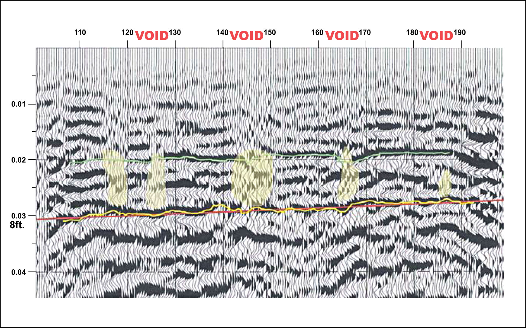
Figure 98. Shear Wave Seismic Section.

Advantages: Providing the seismic source can produce high frequencies, the method can provide good resolution.

Limitations: As with compressional wave seismic reflection the method is quite labor intensive and can require significant data processing.

Resistivity Measurements to Map Fractures

Basic Concept: Resistivity measurements can also be used to locate fracture zones, since these areas often have a lower resistivity than unfractured bedrock. The method and instruments used are described earlier in this section and will not be described here.

Resistivity measurements can be taken with a simple four-electrode array or with the more sophisticated systems that use addressable electrodes, called Automated Resistivity systems. These systems provide an efficient method for measuring the lateral and vertical variations in resistivity and are the preferred system for locating fracture zones. Figure 201 shows the Sting/Swift instrument for taking these measurements.

Figure 201. Sting-Swift Resistivity Measuring System. (Advanced Geosciences, Inc.)

Data Acquisition: With the automated resistivity system, the electrodes and wire connections are made before data recording begins. Once this is done, the data recording parameters and electrode array to be used are entered into the controller, which is then instructed to record the data. Since this system measures resistivity along the profile at a number of electrode spacings, it provides both lateral and vertical variations in resistivity. If long lines of data are recorded, the system is incrementally moved along the line as the survey progresses.

Fracture zones are also located using Azimuthal Resistivity measurements. With this method the electrode array is rotated about its center while taking resistivity readings. However, the method assumes that the bedrock surface is fairly flat and that no resistivity changes occur within the overburden.

Data Processing: The data is transferred from the field data recorder to a computer. Generally no processing is required and the data is loaded into interpretation software.

Data Interpretation: The data can be interpreted using computer software that provides a model whose calculated data fit the field data, thereby providing the variation of ground resistivity both laterally and vertically. A preliminary model is input by the interpreter, and the software then modifies this model until the resulting pseudosection matches that from the field data. The process of obtaining the model whose data fit the field data is called inversion.

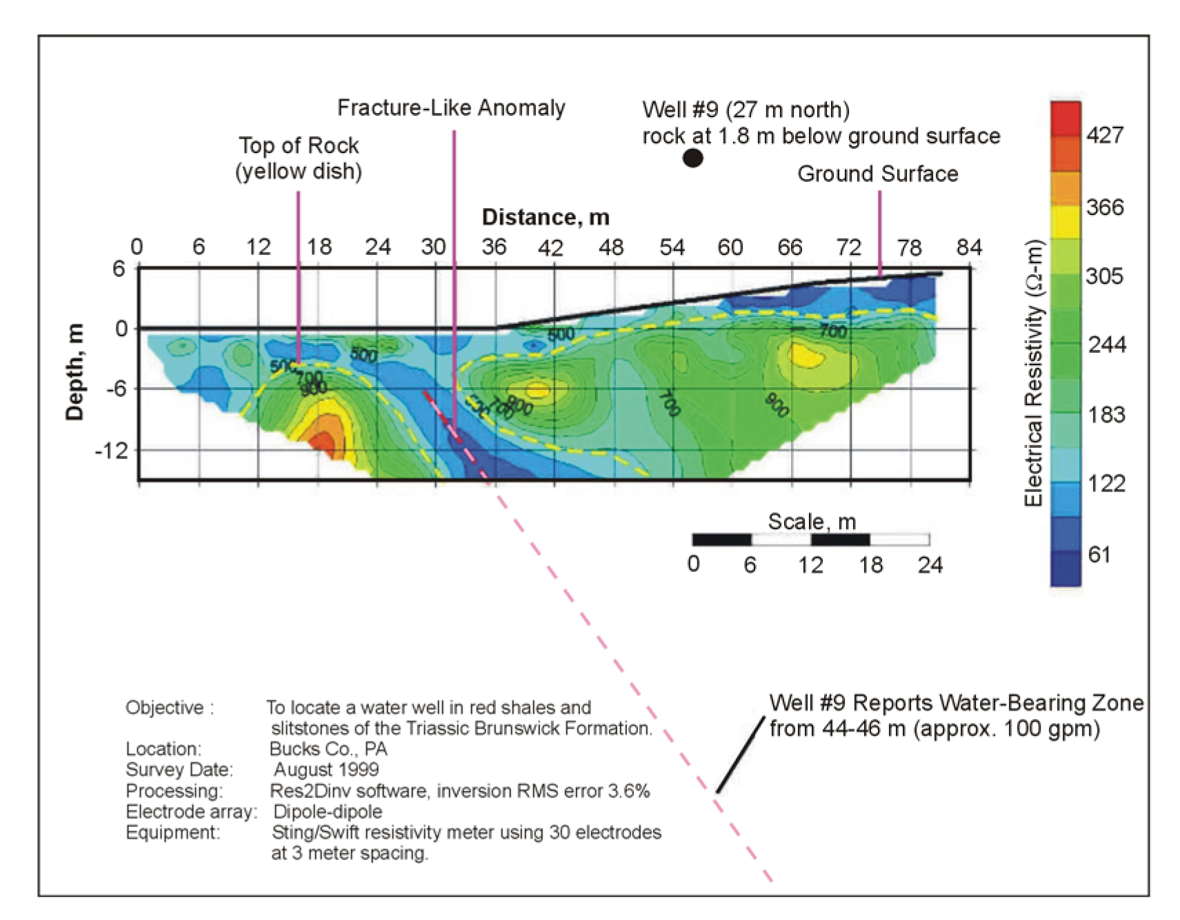
Figure 132. Resistivity measurements used for locating water-bearing fractures. (Quantum Geophysics, Inc.)

Figure 132 shows resistivity data obtained with the Sting/Swift resistivity system that has been inverted to provide a resistivity model showing a depth-versus-distance plot. As can be seen, the water-bearing fracture zone has a significantly lower resistivity than the host rocks.

Advantages: Compared to using a single electrode spacing to measure resistivity along a traverse the Automated Resistivity System provides much more data and allows for a much better interpretation.

Limitations: A resistivity contrast with the host rocks must exist at the fracture zone. Generally, because fracture zones have a higher porosity than unfractured rock, these areas will contain more moisture and have a lower resistivity then unfractured areas. Since electrodes have to be planted in the ground, areas with hard surfaces require more time to place these electrodes. Any grounded structure, e.g., metal fences, will influence the data if they are close to the electrode array. Likewise, buried metal features, e.g., pipes, will also create anomalies.

Geophysical Methods to Map Faults.

Since faults often do not often have clear ground or bedrock surface expressions, techniques used to map the locations of faults need to reach depths beyond the bedrock surface and, therefore, generally need to penetrate to depths greater than about 100 m.

For geophysical methods to be able to locate faults, there must, in general, be some difference in the physical properties of the rocks on either side of the fault. However, the seismic reflection method is able to map faults that do not have significant physical property differences on either side. This method provides detailed mapping of reflectors, and when a fault is present, the continuity of these reflectors is often disrupted. Figure 133 shows a seismic reflection section where faults are imaged.

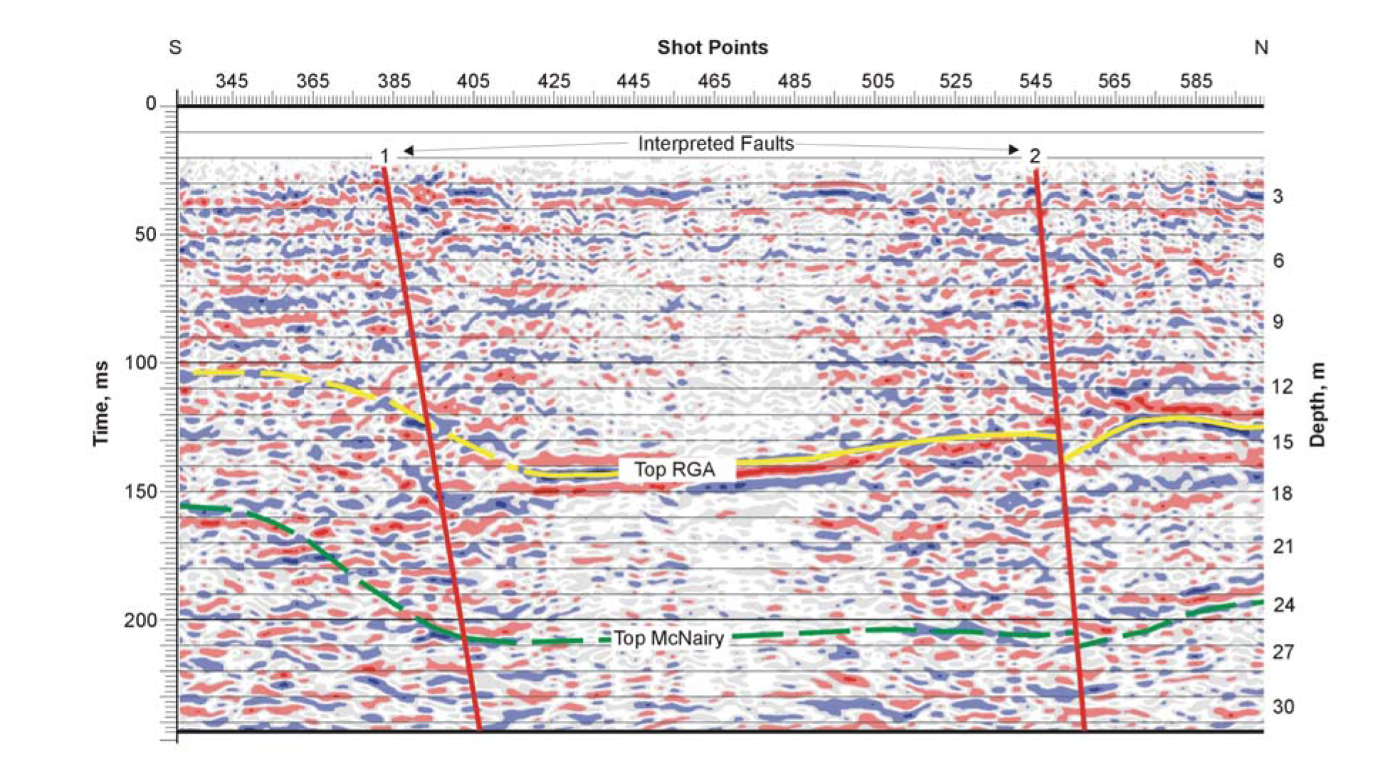
Figure 133. Seismic Reflection section showing faults.

If the fault has placed rocks having different densities next to each other, then the gravitational method may be useful.

A gravity profile across a faulted area will show higher values over more dense rocks and lower values over the rocks with lower densities. In addition to the rocks having different densities on either side of the fault, it is possible that they will also have different resistivities, in which case electrical soundings may be effective. Although resistivity soundings can be used, it is more likely that Time Domain Electromagnetic (TDEM) soundings will be conducted since the fieldwork for these soundings is more efficient than that for resistivity soundings. In addition, the TDEM method provides more depth penetration with less influence from lateral variations in resistivity.