Contamination plumes usually refer to plumes in groundwater. These can arise because of point sources, such as direct discharge of effluent from a pipe or from non-point sources such as the application of pesticides over a wide area, which then seep into the groundwater over time. Plumes can vary in size from quite small to those covering many hectares. In addition to contaminant plumes, geophysical methods are used to find buried trenches, landfill boundaries, and solve other environmental problems.
Often, the original source of contamination contains a suite of chemicals, of which only a small number are contaminants. Because the concentration of contaminants is usually quite small, often measured in parts per million, geophysical surveys can rarely directly detect contaminants. An exception to this might be severe hydrocarbon contamination, where Ground Penetrating Radar (GPR) is sometimes successful. For geophysical methods to be used to detect contamination, other factors must be involved. Some of these are listed below.
The suite of chemicals making up the contamination may be electrically conductive, either because it is acidic or because it contains salts. In this case, the plume is also electrically conductive and can often be detected using electromagnetic methods. If the contaminants are heavier than water, such as dense non-aqueous phase liquids (DNAPL), these chemicals will sink to the bottom of an aquifer. In this case, mapping the topography of the top of the aquitard (maybe a clay layer) that impedes the downward movement of the DNAPL may be valuable. Depending on the geologic conditions, this can be done using several geophysical methods such as electromagnetic, resistivity, refraction seismic, and possibly GPR. It is also possible that the suite of chemicals reacts with clay layers, altering their electrical properties. If that is the case, Spectral Induced Polarization (SIP) may be used. However, this application of the IP method is still being researched and should be considered experimental. Another method that can sometimes be used to detect chemically altered soils and overburden is GPR, since such changes can sometimes affect the dielectric properties of the overburden.
Methods
Electromagnetic
Basic Concept: Electromagnetic methods are used to measure the electrical conductivity of the ground. Several instruments are available to do this including the EM31, EM34, and GEM2. If the vertical distribution of conductivity is needed (or its inverse resistivity), then time domain electromagnetic or resistivity sounding methods can be used. However, usually the most important component in mapping contaminant plumes is to find the aerial extent of the plume. The EM31 instrument is shown in figure 183.
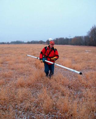
Figure 183. The EM31-MK2 instrument. (Geonics, Ltd.)
Electromagnetic instruments designed to measure ground conductivity use sinusoidal waveform oscillating between 50 and about 20 kHz. The EM31 oscillates just below 10 kHz. This instrument is effective to depths of about 6 m. If conductivity measurements are required to greater depth then the EM34, shown in figure 197, can be used. This instrument can be used to depths greater than 60 m. Three different separations of the two coils can be used providing three different depths of investigation. However, as the depth of investigation increases, the lateral resolution decreases. The EM34, unlike the EM31, cannot be used with one person; two people are required. Data recording is much slower than with the EM31.
All of these instruments measure the bulk electrical conductivity of the ground. Since the conductivity of several different layers may be included in the conductivity measure, the correct technical term for the measured conductivity is apparent conductivity. When discussing EM31 and EM34 data in this website, conductivity is understood to mean apparent conductivity.
Both the EM31 and EM34 use a transmitter and receiver coil, usually used with the coils coplanar. These instruments can be used in two different modes: one is called the vertical dipole mode, and the other is called the horizontal dipole mode. In this mode, the plane of the coils is vertical. In the vertical dipole mode the plane of the coils is horizontal. These two different modes provide different ground responses. In the vertical dipole mode, the instrument is less sensitive to near-surface effects and has the deepest penetration. In the horizontal dipole mode, the near surface ground conductivity has most effect, with deeper layers having much less influence.
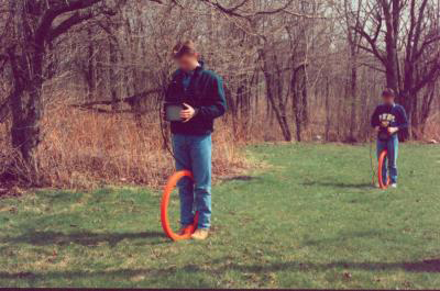
Figure 197. The EM34 being used in horizontal dipole mode. (Geonics, Ltd.)
Data Acquisition: Surveys are conducted by taking readings along lines crossing the area of interest. These lines need to be surveyed to provide spatial coordinates. Readings either are taken at defined stations, or with the EM31, on a timed basis, say every second. The mode (vertical or horizontal dipole) in which the instruments are used depends on the target depth and the objectives. The instruments store the data in memory as it is recorded, allowing it to be downloaded to a computer at a later time.
Example data from an EM survey around a landfill in Oklahoma is presented in figures 198 and 199. Figure 198 shows EM31 data and figure 199 shows EM34 data. Both show conductivity increasing significantly near the landfill boundary.
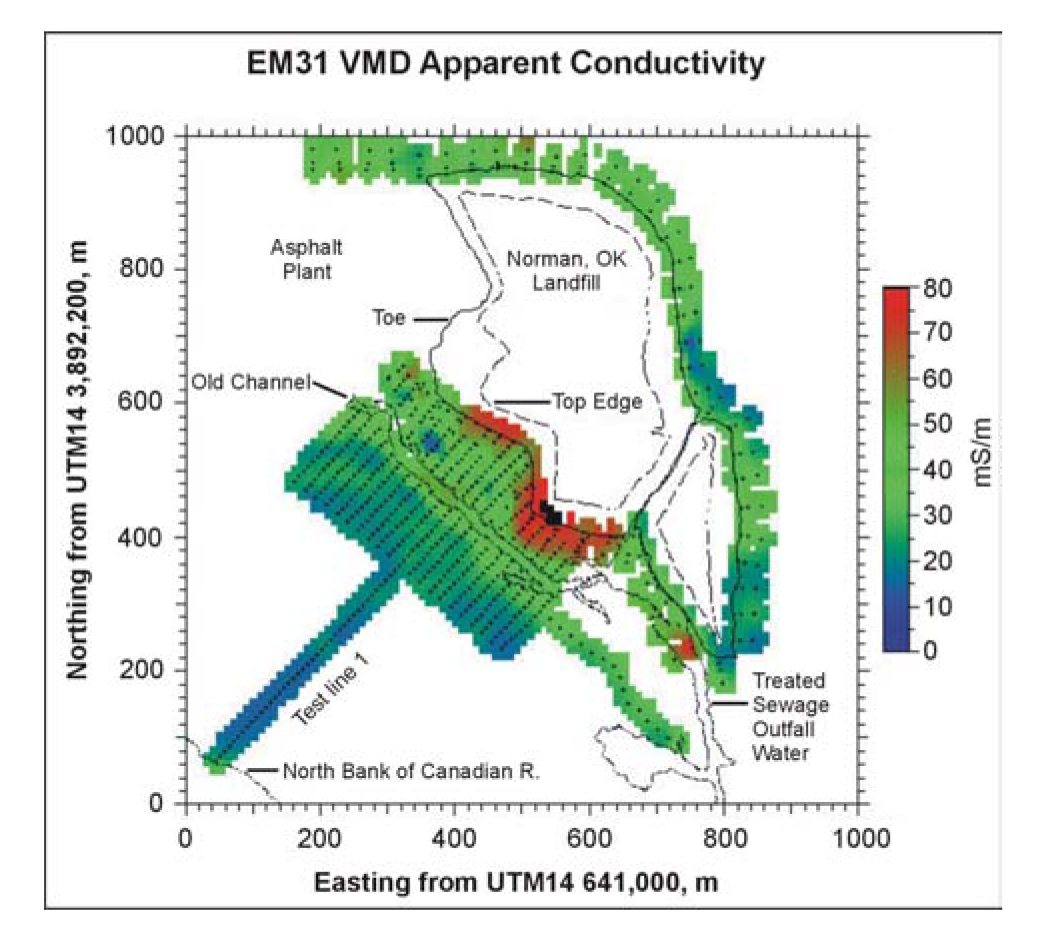
Figure 198. EM31 conductivity data - vertical dipole mode. (USGS)
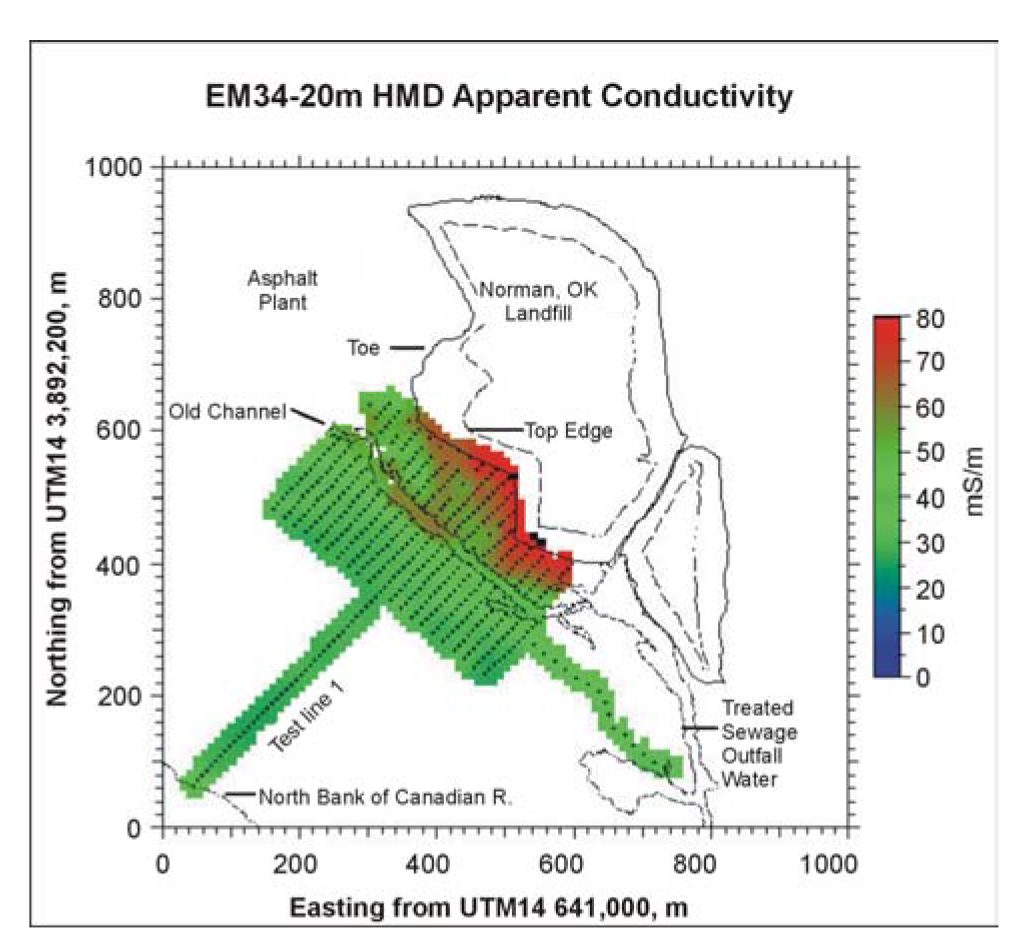
Figure 199. EM34 conductivity data - horizontal dipole mode. (USGS)
The EM31 data were recorded with the instrument in vertical dipole mode (VMD). In this mode, the instrument has a depth of investigation of about 6 m. As can be seen, the conductivity increases from less than 20 mS/m some distance from the landfill to 80 mS/m or more near the landfill boundary. It is likely that the effluent from the landfill has contaminated the groundwater, making it more electrically conductive.
The EM34 data were recorded in horizontal dipole mode using a coil separation of 20 m, giving it an exploration depth of about 15 m, nearly twice the exploration depth of the EM31 data shown in figure 198. The EM34 data show conductivities near the landfill of over 70 mS/m, decreasing to about 30 mS/m some distance from the landfill.
Data Processing: Data processing mostly involves assigning coordinates to each data point. The data are then gridded, contoured, and plotted, producing a map of the measured conductivity at the site.
Data Interpretation: Interpretation is done from this map. Generally, when investigating conductive plumes, this will involve searching for areas of high electrical conductivity. With the EM31, these areas will be fairly well defined since the instrument has a fairly limited area of influence. However, with the EM34, which has a much greater depth of investigation, the lateral resolution is less well defined.
When both the EM31 and EM34 have been used at a site to provide different depths of investigation, more information can be obtained about the site. In the case shown above in figures 198 and 199, the EM34 data, where the depth of investigation was about twice that of the EM31 data, show higher conductivities some distance from the landfill, with values being about 30 mS/m. The EM31 data at this location show values of about 10 mS/m. Clearly, the conductivities are increasing with depth. In addition, the region of high conductivity near the landfill shows a greater aerial extent with the EM34 data. This suggests some of the contaminant plume extends to depths beyond the reach of the EM31 and is, therefore, deeper than about 6 m.
Advantages: The conductivity instruments described above are easy to use and provide efficient field surveys. Although the data is usually plotted and then interpreted, the instruments display the measured conductivity and approximate anomaly locations can be observed during the field survey.
Limitations: Clearly, a conductivity contrast has to occur for the method to be effective. Probably the largest limitation is the influence of surface metal, fences, power lines, and other cultural features. However, if the plume is expected to have a significant aerial extent, local metal interferences will probably be easily recognized from the long wavelength conductivity anomaly from a plume. The EM34 is considerably more cumbersome to use and slower than the EM31. Since it requires two people to operate, the field cost is also greater.
Resistivity
Basic Concepts: Resistivity methods can also be used to map the spatial and vertical extent of plumes, providing they have a resistivity contrast. Resistivity measurements can be obtained using four electrodes placed in the ground. A number of different electrode arrays can be used, several of which are shown in figure 90.
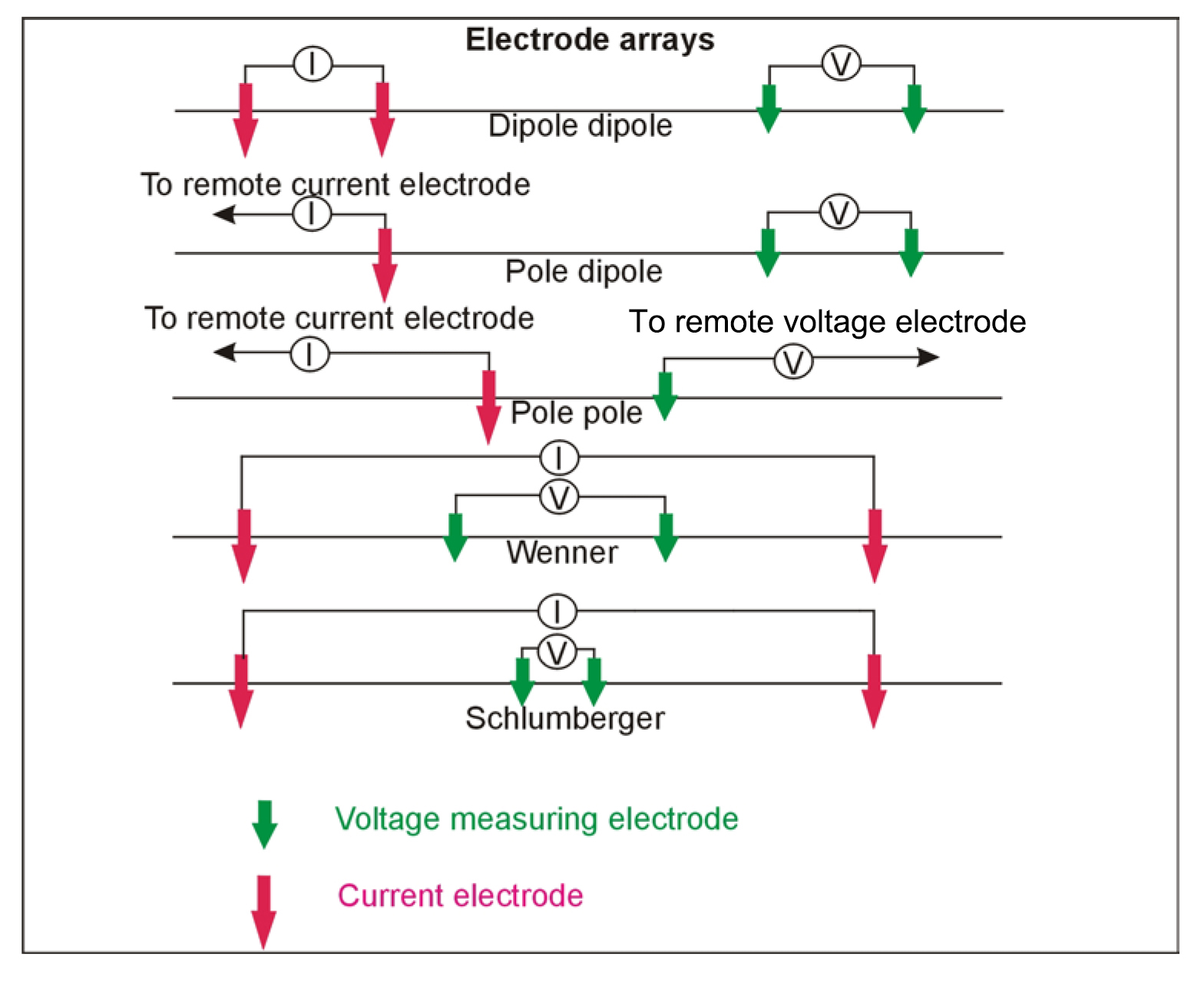
Figure 90. Electrode arrays used to measure resistivity.
These arrays are used for different types of resistivity surveys. The Schlumberger array is often used for resistivity soundings, as is the Wenner array. The pole-pole array provides the best signal but is cumbersome because of the long wires required for the remote electrodes, and it is rarely used. The dipole-dipole array was originally used mostly by the mining industry for Induced Polarization surveys. Readings were taken using several different separations of the voltage and current dipoles providing measurements of the variation of resistivity with depth. Long lines of data were recorded requiring many readings. This array has now become common for resistivity surveys using the automated resistivity systems. If more signal (voltage) is needed than can be provided with the dipole dipole array, the pole dipole array can be used. Resistivity is measured by passing electrical current into the ground using two electrodes and measuring the resulting voltage using the other two electrodes. The apparent resistivity is calculated by multiplying a geometric factor for the array by the measured resistance (voltage divided by current).
These arrays are used for different types of resistivity surveys. The Schlumberger array is often used for resistivity soundings, as is the Wenner array. The pole-pole array provides the best signal but is cumbersome because of the long wires required for the remote electrodes and it is rarely used. The dipole-dipole array was originally mostly used by the mining industry for Induced polarization surveys. Readings were taken using several different separations of the voltage and current dipoles providing measurements of the variation of resistivity with depth. Long lines of data were recorded requiring many readings. This array has now become common for resistivity surveys using the automated resistivity systems. If more signal (voltage) is needed than can be provided with the dipole-dipole array, then the pole-dipole array can be used.
Data Acquisition: Resistivity traverses can be obtained by taking readings using one electrode spacing at regular stations forming a line of data. In this case, the spatial variation of resistivity is obtained. Resistivity data can also be taken keeping the center of the array fixed and expanding the electrode array, thus obtaining data from different depths and forming a resistivity sounding. If the depth to the aquitard is needed, the electrical soundings can be used. An electrode arrangement, lines of current flow, and a resistivity sounding curve are shown in figure 91a.
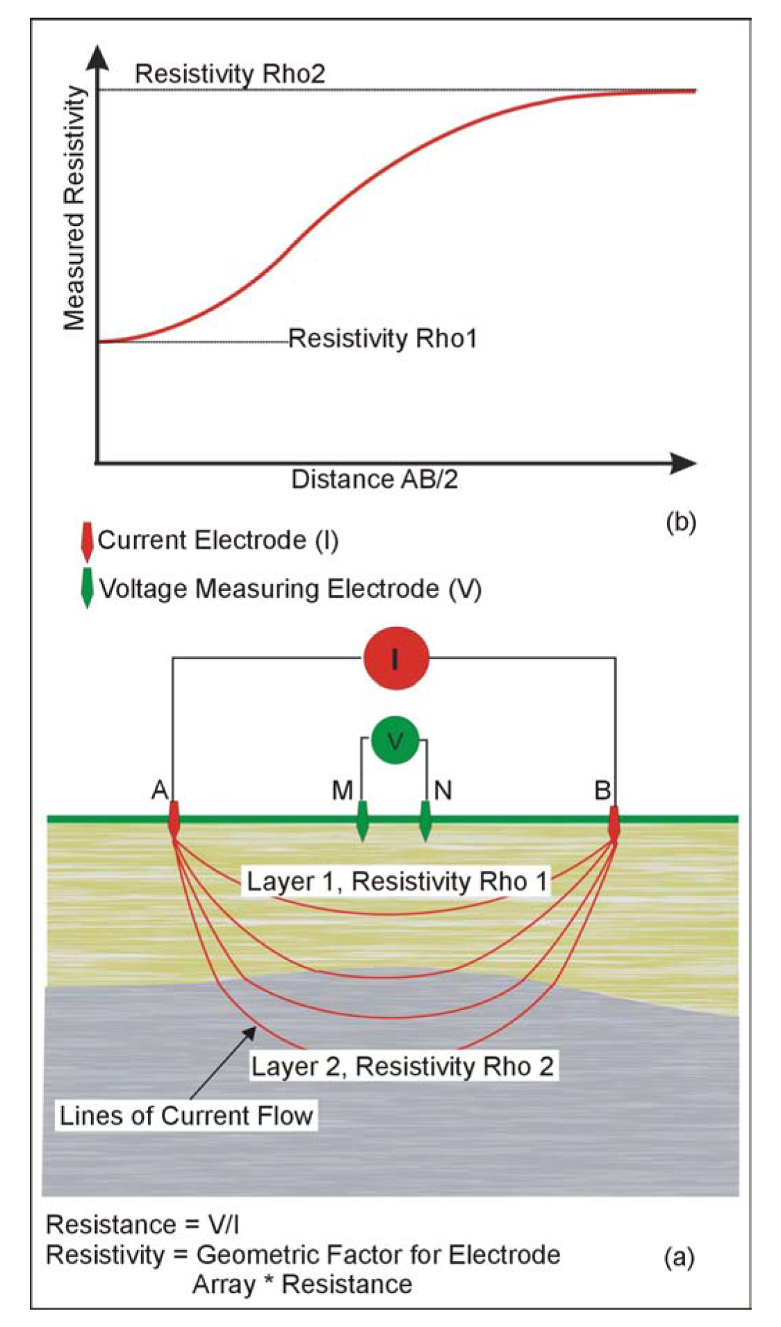
Figure 91. Electrode array for measuring the resistivity of the ground.
In figure 91b, the measured resistivity is influenced by both layer 1 and layer 2. When the electrode spacings are small, the measured resistivity approaches that of layer 1. Likewise, when the electrode spacing is large, the measured resistivity approaches that of layer. By measuring resistivity at a number of electrode spacings, a graph of apparent resistivity against electrode spacing can be drawn. The data can then be interpreted to give the depth to the top of layer 2.
Resistivity traverses using one electrode spacing are rarely used since EM methods can provide very similar results with much greater efficiency. If resistivity traverse measurements are made with many electrode spacings, as is usually the case with the automated resistivity systems discussed below, the variation of resistivity with depth can also be obtained.
Data Processing: Usually little processing is required apart from removing bad data points.
Data Interpretation: Resistivity soundings are interpreted by using software that calculates the expected field curve from a resistivity model. The program then modifies this model until the calculated field data matches the actual field data. This process is called inversion.
Advantages: Resistivity soundings will mostly be used to find the vertical extent of a contaminant plume, providing there is a resistivity contrast associated with the plume.
Limitations: As stated under Advantages, the plume must have a resistivity contrast in order to be detected.
Another fairly recently developed instrument for measuring the resistivity of the ground is called the Ohm-Mapper, manufactured by Geometrics in California. This instrument has a series of electrodes on a cable that is dragged at a slow pace along the ground. Current is induced into the ground, and the resulting voltages measured. The electrodes are capacitively coupled to the ground, and both transmit current into the ground and measure the resulting voltage. The Ohm-Mapper instrument being towed along the ground surface is shown in figure 200.
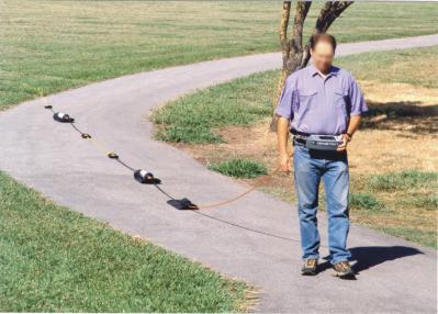
Figure 200. The Ohm-Mapper. (Geometrics, Inc.)
Automated Resistivity Systems
Basic Concept: Taking resistivity readings using many electrode spacings can be done using instruments that use automated resistivity recording, making resistivity data collection quite efficient. These systems allow the electrodes to be placed in the ground and connected to the data recorder prior to recording data. When setup is complete, the recorder is programmed with the data recording parameters to use and then automatically collects the data according to a pre-programmed schedule. One system that does this is illustrated in figure 201.
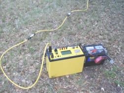
Figure 201. Sting-Swift Resistivity Measuring System. (Advanced Geosciences, Inc.)
An example of data recorded using this system is shown in figure 202.
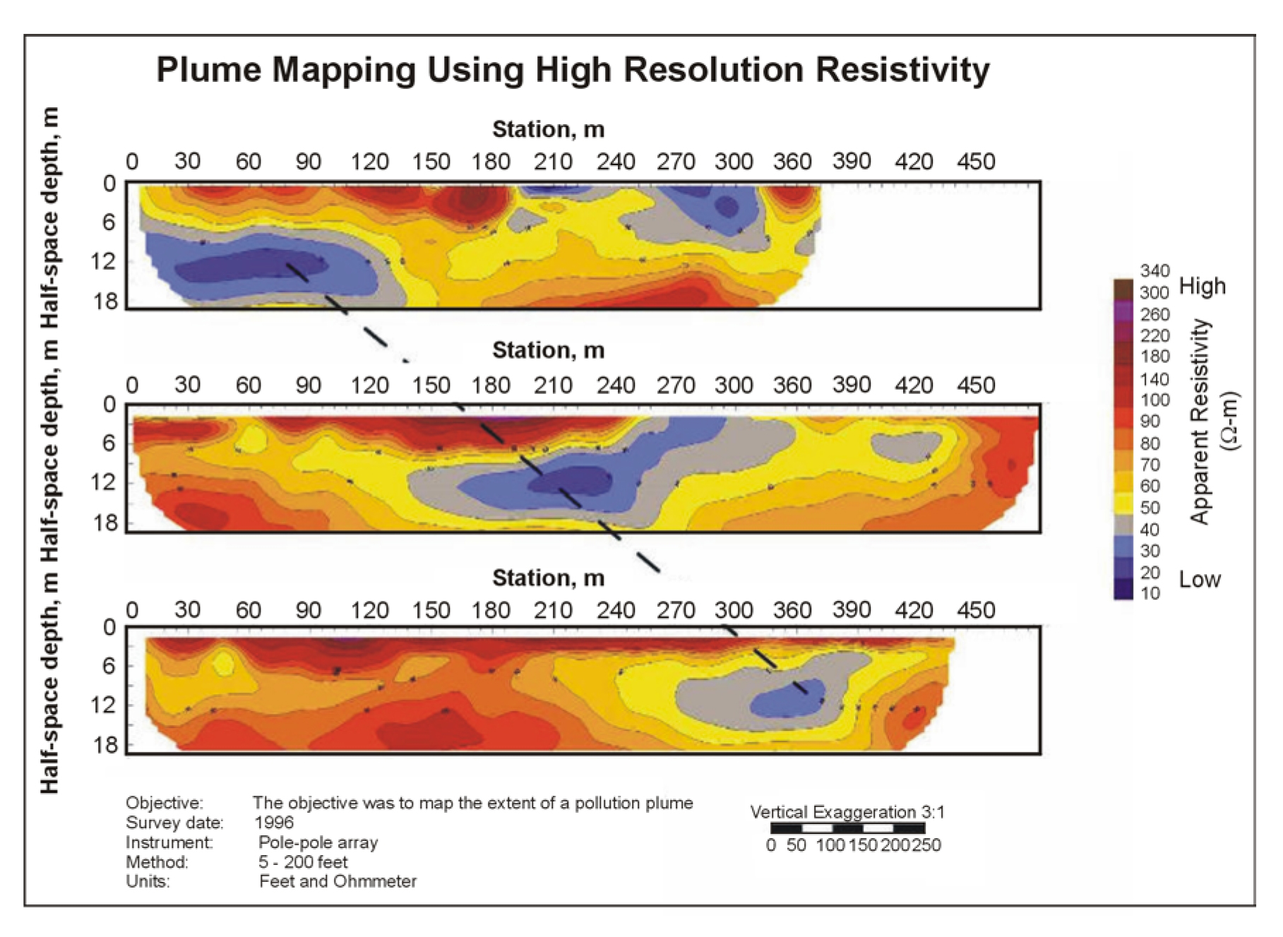
Figure 202. Example data recorded with the Sting-Swift System. (Advanced Geosciences, Inc.)
Data Acquisition: The electrodes are laid out along a straight line and connected to the data recorder. This is then programmed with the particular electrode array to use and instructed to take the data. Figure 202 illustrates the detail that can be obtained when resistivity measurements are taken using several electrode spacings along a traverse. The data are plotted in the form of a pseudosection, in which the data from small electrode spacings are plotted near the ground surface line, and those from large electrode spacings are plotted at greater distances vertically beneath the ground surface line, thus simulating depth. In this case, a low resistivity region on each of the three lines marks the occurrence of a contamination plume. The data can also be modeled to give the depth of the source of the resistivity anomalies.
Data Processing: Resistivity data require little processing although bad data points may be removed.
Data Interpretation: Interpretation may be visual, or modeling can be done to provide the spatial distribution of the source of the anomaly along with its depth. This is usually done using software that modifies a preliminary resistivity/depth model until the output data from the model matches the field data, a process called inversion.
Advantages: The Automated Resistivity System records a significant amount of data quite efficiently. Fairly detailed interpretations can be done using this data.
Limitations: Resistivity methods can be used to spatially map contaminant plumes. They rely on the plume having a different resistivity (or conductivity) to that of the surrounding, uncontaminated areas. Essentially, if electromagnetic methods can be used to map a plume, then resistivity methods can probably also be used.
If a single electrode spacing is used, the resistivity measuring system is rather slow, and EM methods are a better choice. However, if an automated resistivity system is used, much more data are obtained, and a better interpretation can be produced. Clearly, the resistivity method will be difficult if the ground is hard or if there are areas of concrete or asphalt, making electrode placement difficult.
If grounded metal objects, such as metal fences, are close to the electrode array being used, the data will be influenced by these metal features. Below ground, metal objects such as metal pipes will also influence the data.
Ground Penetrating Radar
Basic Concept: Ground Penetrating Radar (GPR) can be used to map contaminant plumes. However, the method is fairly site specific, and care needs to be taken that the site conditions are appropriate for the GPR method.
The depth of investigation of GPR depends on the soil conditions. A saturated soil with significant clay will severely limit the penetration of the method. Ideal conditions are unsaturated, clay-free soils. Depth of penetration also depends on the frequency of the signal. Different antennas provide different frequencies, which range from about 25 MHz to 2700 MHz. A low-frequency antenna (signal) will provide the best penetration depth but has the lowest resolution.
The GPR instrument consists of a recorder and a transmitting and receiving antenna (see figure 112).
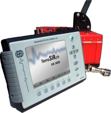
Figure 112. Ground Penetrating Radar instruments. (Geophysical Survey Systems, Inc.)
When the GPR signal reaches an object, or interface, with different dielectric properties, part of the wave is reflected back to the ground surface, where it is recorded by the receiving antenna. Several companies manufacture GPR equipment. These include Geophysical Survey Systems, Inc (GSSI), GeoRadar, Inc, Mala GeoScience, and Sensors and Software Inc.
The 100 MHz antenna is (figure 113) suited for deeper applications to depths of about 20 m. This antenna can be used to locate contaminant plumes.
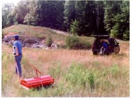
Figure 113. Ground Penetrating Radar antenna (100 MHz) used in survey. (MALA GeoScience USA,Inc.)
Data Acquisition: GPR surveys are conducted by pulling the antenna across the ground surface at a normal walking pace. The recorder stores the data as well as presenting a picture of the recorded data on a screen.
Data Processing: It is possible to process the data, much like the processing done on single-channel reflection seismic data. Processes that can be applied include distance normalization, horizontal scaling (stacking), vertical and horizontal filtering, velocity corrections, and migration. However, depending on the data quality, processing may not be done since the field records may be all that is needed to observe the contamination plume.
Data Interpretation: Data interpretation is mostly visual. If the depth to an anomaly is required, then the speed of the GPR signal in the soil at the site has to be obtained. This can be estimated from ts showing speeds for typical soil types or it can be obtained in the field by conducting a small traverse across a buried feature whose depth is known.
Figure 203 shows the results of a GPR survey over a hydrocarbon plume. The plume is easily observed from the signal attenuation and lack of spatial coherence caused by the plume.
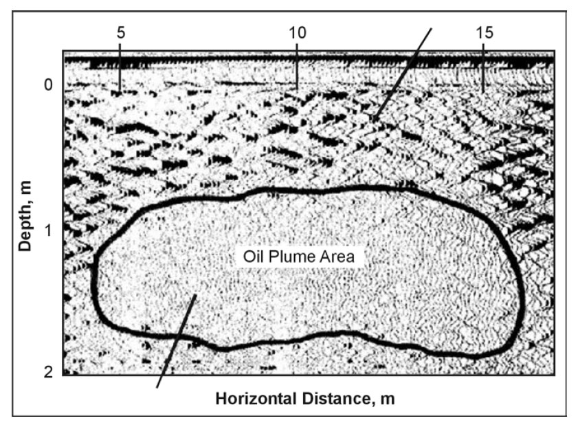
Figure 203. Ground Penetrating Radar data over a hydrocarbon plume. (GeoSurvey)
Advantages: GPR surveys are fairly easy to conduct and different antenna can be tested if the anomaly resolution or depth penetration are insufficient.
Limitations: Probably the most limiting factor for GPR surveys is that their success is very site specific and depends on having a contrast in the dielectric properties of the target compared to the host overburden, along with sufficient depth penetration to reach the target. Surveys near high-powered radio frequency antenna may also inhibit subsurface data collection.
Induced Polarization
Basic Concept: Induced Polarization (IP) is an electrical method that measures the change in the measured resistivity of the ground with frequency. All of the electrode arrays used to measure resistivity (see figure 90) can also be used to measure IP. In fact, when measuring IP, resistivity is also measured. There are two methods used to obtain IP data: one called time domain, and the other called frequency domain. In time domain, a constant current is passed into the ground using two of the four electrodes. This current is then rapidly switched off. During this off time, the remaining two electrodes measure the resulting voltage. If an IP effect is present, the voltage across these electrodes will not suddenly return to zero as the current is turned off, but will decay to zero over a period of time, usually within a few seconds. In frequency domain the resistivity of the ground is measured at different current/voltage frequencies.
Figure 90. Electrode arrays used to measure resistivity.
Figure 110 illustrates the electrode array and the current and voltage waveforms showing the voltage decay after the current is turned off. Simple IP measurements usually integrate the IP voltage over a specified time period, say T1 and T2 (see figure 110), providing a single number, called chargeability that is a measure of the IP response. However, if the current and voltage waveforms are recorded, a Fourier transform can be applied to the data, and the variation of resistivity with frequency obtained, called Spectral Induced Polarization (SIP).
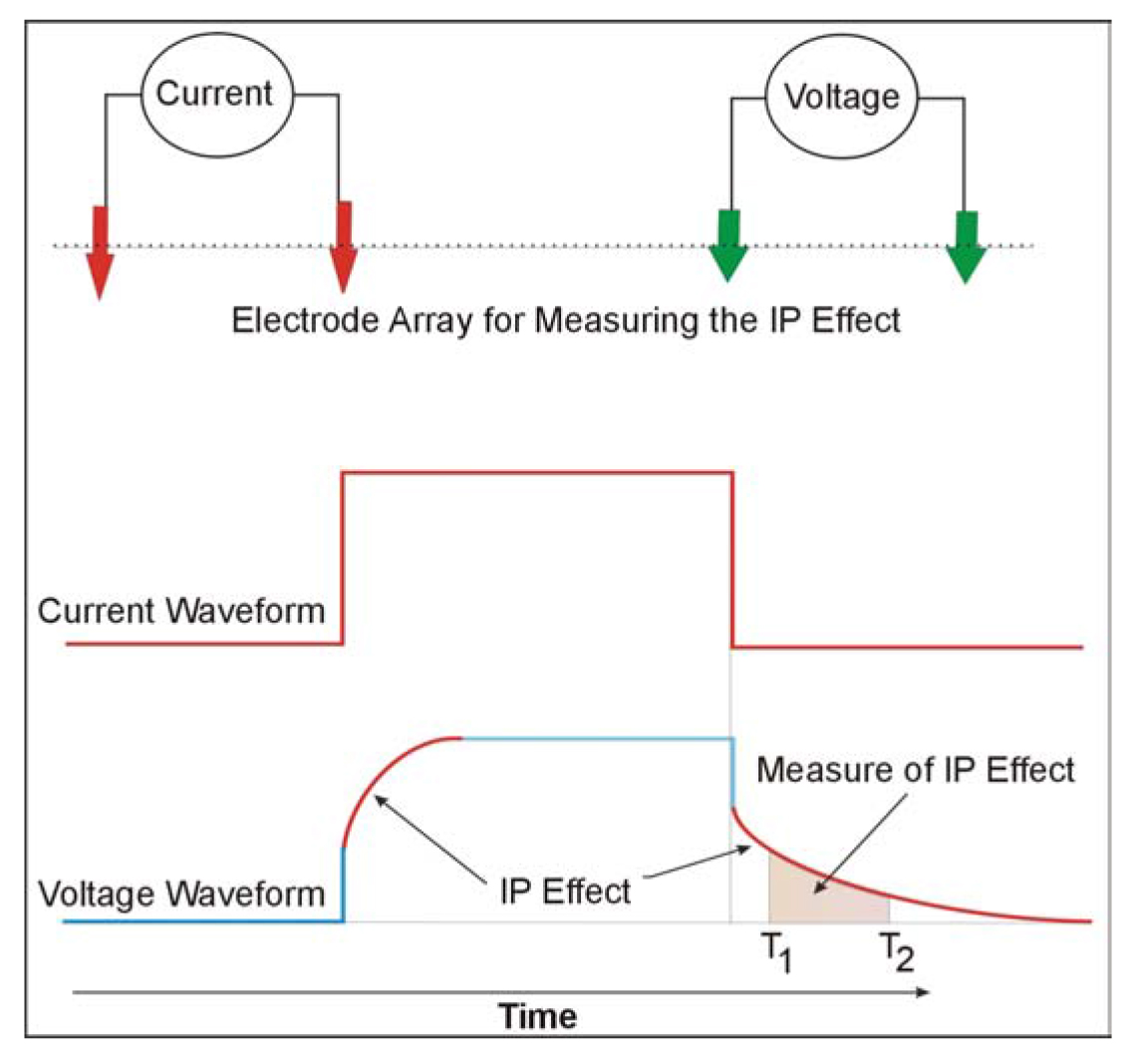
Figure 110. Induced Polarization waveform.
The use of the IP method for mapping contamination and plumes is essentially still being researched. This is especially true for the SIP method. The method relies extensively on the influence that chemical contaminants have on clay. Clay often has a natural IP response, and this is sometimes changed by the chemicals comprising the plume.
Data Acquisition: Induced Polarization surveys are conducted much like resistivity surveys. Readings are taken at discrete stations to form lines of data crossing the area of interest. The automated recording system discussed previously for resistivity measurements can also be used to record IP data. Generally, the dipole dipole electrode array is used.
Data Processing: If digital data are obtained at several frequencies, the variation of IP response with frequency is obtained. In the time domain, the current and voltage waveforms have to be digitally recorded and a Fourier analysis of the data be performed providing the variation of resistivity with frequency. The variation of IP response with frequency is called Spectral Induced Polarization and provides more interpretable information than the simple IP measure discussed above. However, this is still being researched and is rarely used as a production method.
IP data field is usually plotted in the form of a pseudosection where data from the smallest dipole spacing are plotted near the ground surface line and those from the larger dipole spacings are plotted at a greater vertical distance from the ground surface line, thus simulating a plot of data against depth. Both the resistivity data and the IP data (chargeability) are plotted on pseudosections.
Data Interpretation: Often the pseudosection data is interpreted visually, using standard model curves of specific geologic structures. However, it is also possible to use software to invert the data, thereby providing a geologic model whose calculated values (resistivity and chargeability) fit the field data.
Advantages: This method is not commonly used to map contaminant plumes although it may provide some useful information in some cases.
Limitations: The IP method is quite labor intensive and requires electrodes be inserted into the ground. Generally, more current is needed than for a resistivity survey to the same depth since the IP voltages can be quite small; hence, the resistance of the electrodes to ground (contact resistance) needs to be as low as possible. This may require watering the electrodes to improve the electrical contact between the electrodes and ground (reduce the contact resistance). If the ground surface is hard, then inserting the electrodes may be difficult.
Grounded metal structures such as fences that are local to the measuring site can significantly influence the data, possibly making the data uninterpretable.
Electromagnetic Methods to Map Aquitard Topography
Basic Concept: The EM31 and EM34 can be used to map variations in the depth to the top of an electrically conductive aquitard. This may be useful when DNAPL's are the contaminant, and it is suspected they may have pooled in a depression on top of an aquitard. The EM31 and EM34 instruments are shown in figures 183 and 197, respectively, and their mode of use is described previously. If depths to the aquitard are needed, and the aquitard is less than about 30-m deep, then resistivity soundings can be used to convert the conductivity data to depth data. This can be done by performing soundings at regular intervals along the traverse and using the interpreted depths to convert the conductivity values from the EM31 or EM34 data to depths.
Figure 183. The EM31-MK2 instruments. (Geonics, Ltd.)
Figure 197. The EM34 being used in horizontal dipole mode. (Geonics, Ltd.)
Figure 204 presents a diagram showing the DNAPL resting in a depression on top of an aquitard. In this case, a relatively low conductivity overburden rests on a conductive aquitard, with DNAPL resting in the depression on top of the aquitard. Providing the EM instrument used penetrates well into the aquitard, the measured conductivity will be significantly influenced by the conductivity of the aquitard. Conductivity measurements taken when the aquitard is near the ground surface will show high values, whereas those taken when the aquitard is deep will show low values. Thus, a traverse across the depression in the aquitard will image the depression, as shown in the illustration. The DNAPL's probably have a low electrical conductivity and will therefore have little influence on the data.
Data Acquisition: Conductivity surveys designed to map the topography of a conductive unit at depth (an aquitard) will normally be conducted along lines crossing the area of interest. Several lines should be surveyed and conductivity data recorded. These lines will need to be surveyed in order to draw a map of the final data.
Data Processing: Usually, little processing is done to the data, although bad data points may be removed.
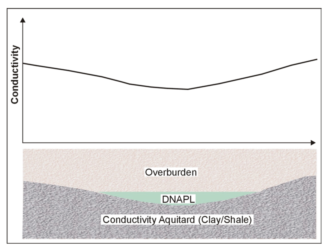
Figure 204. Using conductivity to map aquitard topography.
Data Interpretation: Interpretation is often visual, looking for the conductivity lows for deeper sections of the conductor. If resistivity soundings have been recorded, the conductivity values can be converted to conductivity versus depth.
Advantages: Measuring the ground electrical conductivity with the instruments described above is easy and field production is quite fast.
Limitations: The aquitard layer has to be thick enough to have a significant influence on the conductivity readings. In addition, it has to be more conductive than the overburden, which should usually be the case. If shallower conductive layers occur, or possibly fade in and out spatially, this may obscure the interpretation of the deeper conductive layer. Local metal, either above or below the ground surface, will influence the measured conductivity data.
The method provides lateral variations in conductivity, but only very limited depth determinations. If these are needed, then other methods will have to be used.
Seismic Refraction to Map Aquitard Topography
Basic Concept: The seismic refraction method can be used to map the top of the aquitard if it has a velocity greater than that of the overburden.
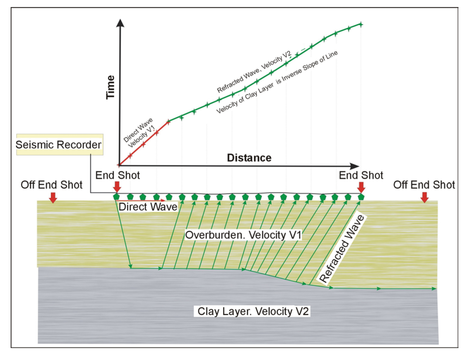
Figure 205. Seismic refraction principles.
In this method, illustrated in figure 205, a seismic wave is created (hammer blow to the ground or explosive shot), and the wave travels into the ground until it reaches a higher velocity layer. At this boundary, part of the energy travels along the boundary and some is transmitted through the boundary to greater depths. The wave traveling along the boundary continually refracts energy back to the ground surface where it is detected by geophones. The seismic recorder records these geophone signals. Several shots are recorded at different distances along the geophone spread. A time-distance graph is constructed from these data, as shown in figure 205, and is interpreted to give the depth to the refractor. The depth of investigation depends on the seismic source used. A hammer and base plate may be able to penetrate to 15 m, whereas a black powder charge buried at a depth of about 0.75 m may provide penetration to about 30 m. Both compressional and shear waves can be recorded with this method, although compressional waves are mostly used for mapping bedrock topography.
Data Acquisition: The design of a seismic refraction survey requires a good understanding of the expected bedrock and overburden. With this knowledge, velocities can be assigned to these features and a model developed that will show the parameters of the seismic spread best suited for a successful survey. These parameters include the length of the geophone spread, the spacing between the geophones, the expected first break arrival times at each of the geophones, and the best locations for the off end shots. Knowing the expected first break arrival times is also helpful in the field, where field arrival times that correspond fairly well to expected times helps confirm that the spread layout has been appropriately planned and that the target layer is being imaged.
Data Processing: The first step in processing/interpreting refraction seismic data is to pick the arrival times of the signal, called first break picking. A plot is then made showing the arrival times against distance between the shot and geophone. This is called a time-distance graph, as shown in figure 205 for two-layered ground (overburden and refractor).
The red portion of the time-distance plot shows the waves arriving at the geophones directly from the shot. These waves arrive before the refracted waves. The green portion of the graph shows the waves that arrive ahead of the direct arrivals. These waves have traveled a sufficient distance along the higher speed refractor (bedrock) to overtake the direct wave arrivals.
Data Interpretation: There are several methods of refraction interpretation. One of the most common methods is called the Generalized Reciprocal Method (GRM) that is described in detail in the Geophysical Methods section. A brief and simplified description of the GRM method is presented below. Figure 206 shows the basic rays used for this interpretation.
The objective is to find the depth to the bedrock under the geophone at D. This is done using the following simple calculations. The travel times from the shots at A and G to the geophone at D are added together (T1). The travel time from the shot at A to the geophone at G is then subtracted from T1. Figure 207 shows the remaining waves after the above calculations have been performed. These are the travel times from C to D added to the travel times from E to D subtracting the travel time from C to E. The sum of these travel times can be shown to be approximately the travel time from the bedrock at H to the geophone at D. Since the velocity of the overburden layer can be found from the time distance graph, the distance from H to D can be found giving the bedrock depth.
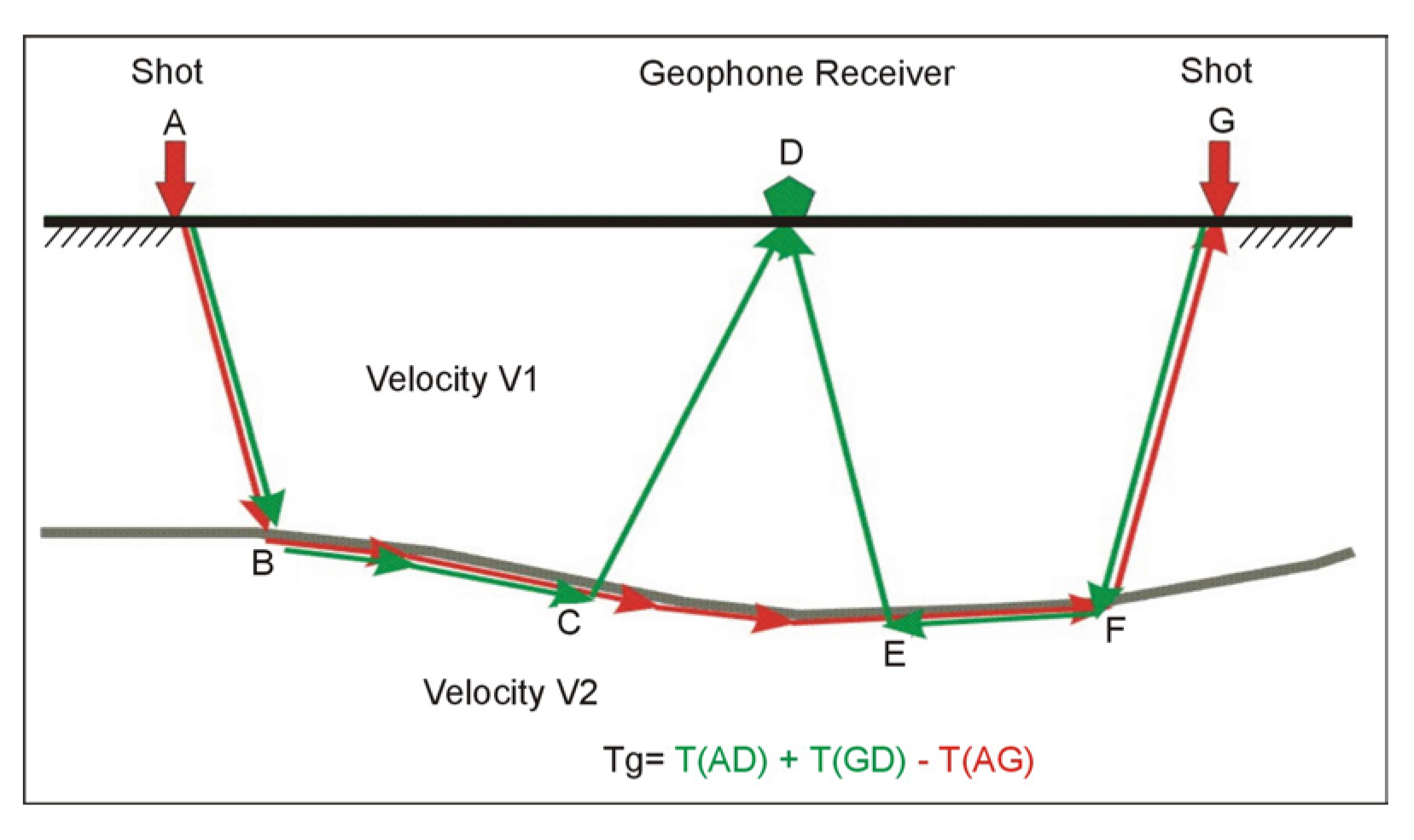
Figure 206. Basic Generalized Reciprocal Methods interpretation.
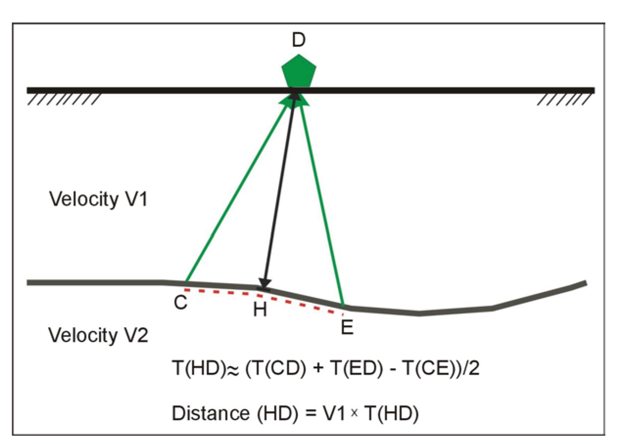
Figure 207. Generalized Reciprocal Methods interpretation.
An example of the results from a seismic refraction survey is presented in Figure 208. Although this example does not map aquitard topography, it does show the field data and results from a seismic refraction survey. The upper figure shows the travel time graph, illustrating the time that the seismic waves take from the shot to each geophone. The second graph presents the interpreted seismic velocity and the third graph shows the interpreted bedrock section.
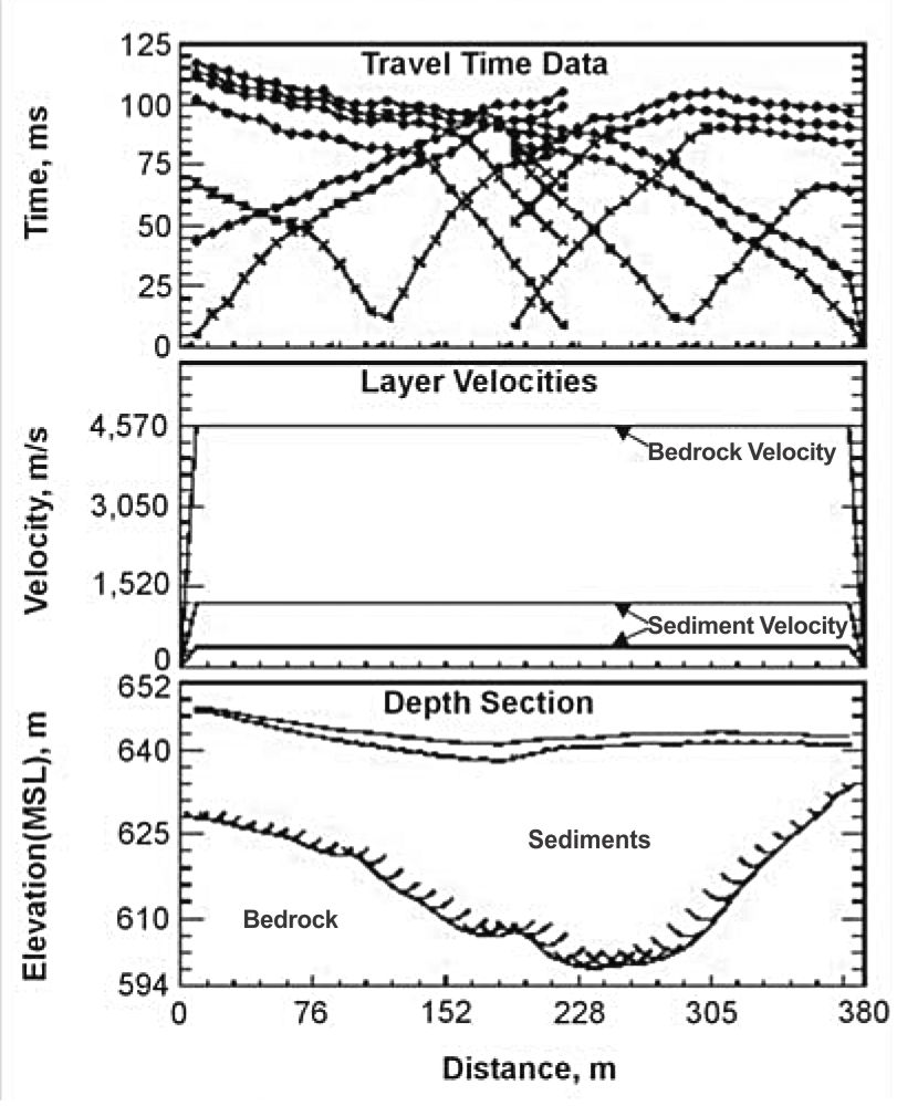
Figure 208. Example of a seismic refraction interpretation.
Advantages: Providing the velocity of the bedrock is greater than that of the overburden, the refraction seismic method can provide good estimates of the bedrock depth, and hence topography.
Limitations: Probably the most restrictive limitation is that each of the successively deeper refractors must have a higher velocity than the shallower refractor. However, for determining the topography of a fairly shallow (less than 15 m deep) clay layer, this is probably not a significant limitation, providing the clay layer has a higher velocity than the overburden. If the water table is in the overburden and close to the bedrock, this may obscure the bedrock arrivals since saturated soils have a higher velocity than unsaturated soils.
Local noise, for example traffic, may obscure the refractions from the bedrock. This can be overcome by using larger impact sources or by repeating the impact at a common shot point several times and stacking the received signals. If noise is still a problem, then a larger energy source may be required. In addition, since some of the noise travels as airwaves, covering the geophones with sound-absorbing material may also help to dampen the received noise.